Our Perception of Risk

May 12, 2024

by Stephen Stofka

This week’s letter is about our perception of investment risk, and the subjective and objective aspects of risk evaluation. Our journey will take us several hundred years in the past and several decades into the future. The triennial survey of consumer finances indicated that less than half of people nearing retirement have $100,000 in liquid financial assets like savings accounts, stocks and bonds. Half of all working households have no savings, leaving them vulnerable to specific circumstances or a general economic shock. In our 20s, retirement looks remote with many years of work ahead of us. As we near retirement, we look in the other direction, to the past, and wish we had saved more. We confront the reality that we feel today’s needs more urgently than tomorrow’s possibilities. A $100 saving has a $100 impact on our current consumption but is only a faint light compared to the many thousands of dollars we will need in the future. We may not understand the underlying mechanism of saving.

We rely on what is visible to our senses to develop a flow of causality. We press on our car’s gas pedal and go faster, convinced that our action is adding more fuel to the engine. What the pedal controls is not fuel, but the air flow leading into the combustion chambers of the engine. The increased flow of fuel occurs in response to the change in air pressure. Prior to the 1980s cars used carburetors and mechanically employed this process called the Bernoulli principle, the idea that faster moving air induces a lower air pressure, a vacuum effect that sucks fuel toward the engine. Today’s fuel injection systems use air flow sensors that direct a computer to adjust the fuel flow. So, what does this have to do with risk?

Bernoulli’s principle is named after Daniel Bernoulli, the son of a noted Swiss mathematician and the nephew of Jacob Bernoulli, a 17th century mathematician who developed foundational concepts in probability like the Law of Large Numbers. Jacob maintained that people perceived risk in two ways. The first was an objective measure, an estimate of the probability of some event. The second was a subjective measure that depended on each person’s wealth, an inverse relationship. The first is visible, like the pressing of a gas pedal. The second is less visible, like the change in air pressure. Imagine that two people agree to flip a fair coin for a $100 bet. Person A has $1000 in her pocket; person B has $200. The loss or gain of $100 represents only 10% of A’s wealth, but 50% of B’s wealth. Even though the chance of winning or losing is the same for each person, they perceive the outcome differently. Peter Bernstein (1998) presents an engaging narrative of Jacob’s ideas in his book Against the Gods. His trilogy of books on the history of investing, risk and gold will inform and entertain interested lay readers.

Jacob may have identified one subjective element in each person’s evaluation of risk, but a person’s stock of wealth is not the only basis for a subjective estimate of risk. There are retired folks with accumulated savings of a million dollars who keep their money in savings accounts or CDs because they perceive the stock and bond markets as risky. A $10,000 loss in the stock market is only 1% of a million-dollar wealth yet some people perceive that loss in absolute dollars, magnifying the effect of a $10,000 loss. They regard the stock and bond markets as different versions of a casino. That same person might give $10,000 to a grandchild for college or to help buy a car, reasoning that there is an exchange of something that a person values for the $10,000. A person has no sense of receiving anything when their stock portfolio shows a $10,000 decrease. The stock market should have to pay an investor for using her investment, not the other way around. Such perceptions are confirmed during crises when the stock market loses 50% of its value.

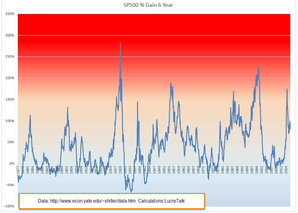
Is an investment in the stock market like putting a quarter in a slot machine? Another perspective: an investor is like an investment company selling insurance to the stock market. A century of data shows that the probability of a loss in the stock market in any specific year is about 25%, according to an article in Forbes. In 70 years, the SP500 has doubled every seven years on average. An insurance company relies on Jacob Bernoulli’s Law of Large Numbers and diversification to manage risk. An investor, like any insurance company, will experience losses in some years. In last week’s letter (see note below) I wrote about surplus as a key dynamic factor in market transactions. In most years, an investor with a surplus of funds can “sell” those funds to the market and reap a gain.

Like risk, values in the stock market are based on both objective and subjective components. Sales, profits, dividends and efficiency help anchor a stock’s price movements as objective measures of value. Price responds to changes in these variables. Objective measures also include the variation in a company’s stock as a precise measure of uncertainty. There are various less precise but objective measures of economic and financial risk. Subjective measures include an investor’s need for liquidity, the ability to turn an investment into cash without impacting the price. An investor’s wealth can act as a cushion against fear of loss, a subjective measure discussed earlier.

Index funds have grown in popularity because they take advantage of Jacob Bernoulli’s Law of Large Numbers. By owning partial shares in many companies, an investor reduces the risk exposure to the variation in the fortunes of one company. The SEC might open an investigation into the ABC company, or the company loses an important overseas market, or the company reveals that the profit margins on some of its popular products are decreasing. To an index fund investor, a 10% decrease in that company’s stock price may be barely noticeable. The investor still has a risk of a change in general conditions, like a pandemic, but has dramatically reduced the risk of local conditions specific to one company.

Investors in Bitcoin do not act as an insurance fund for Bitcoin companies who mine Bitcoin. The miners have the surplus and are the sellers of Bitcoin. In the secondary market, the sellers of access to the digital currency market are the two dozen or so ETFs that allow investors to buy interest in a fund that owns bitcoin. Price movement is like a tailless kite flying in a breeze, responding mostly to price forecasts, a characteristic of some derivatives markets. The only objective measure of value and risk is the number of Bitcoin in circulation and the reward for mining new Bitcoin. Bitcoin’s price movement has a high volatility greater than 50% because there is little economic activity that anchors the variation in Bitcoin’s price. Despite the high volatility, an asset manager at an ETF fund makes the case for investing a few percent of a portfolio in a bitcoin ETF. As in our earlier example, the loss or gain depends on the current state of one’s savings.

Understanding the two aspects of risk perception, the objective and subjective, can help us manage our personal risk profile. Through research or the advice of a financial consultant we can understand the objective measures of portfolio risk but there are subjective elements unique to our personal history and disposition. The fear of having to be in a long-term care facility may influence our yearning for safety, regardless of our current health. A parent or relative may have had a similar experience and our primary concern is the protection of our portfolio value. We may feel fragile after the loss of our entire savings in a business venture. We can only become comfortable with our apprehensions by becoming familiar with them.

Next week I will look at our perceptions of other significant factors in our lives, particularly inflation.

/////////////

Photo by 𝓴𝓘𝓡𝓚 𝕝𝔸𝕀 on Unsplash

Keywords: stocks, bonds, risk, investment

Bernstein, P. L. (1998). Against the Gods: the Remarkable Story of Risk. John Wiley & Sons.

In last week’s letter I wrote about surplus as a key dynamic factor in market transactions. A seller of a good or service has a surplus which it values less than the buyer. However, the seller’s cost, including opportunity cost, is more than the cost to the buyer. These two ratios of benefit and cost find an equilibrium in the market that depends on the type of good or service and general conditions.

https://etfdb.com/themes/bitcoin-etfs/

https://www.vaneck.com/us/en/blogs/digital-assets/the-investment-case-for-bitcoin/

Price Illusion

January 8, 2023

by Stephen Stofka

This week’s letter is about price illusions. The past two weeks I have written about the need to sort through past events to find the lessons. The past is a teacher, not a goal. Those who idealize and revere the past must eventually be swept down the drain of time. During this week’s struggle to elect Kevin McCarthy as House Speaker, the more conservative members of the Republican Party voiced their desire to return the country to the past of more than a hundred years ago when the population of 112,000,000 was a third the current size. Instead of learning from the past, we often use elements of history to tell a story. We discard events that do not fit our narrative. Historical analysis serves political interests. Asset analysis suffers from similar distorting strategies.

Technical analysis studies price movements with little regard for the circumstances that prompted the supply and demand, the buying and selling that underlie those movements. I will pick a few such variants at random. Elliott Wave theory bases its interpretation of price movement on the Fibonacci sequence of numbers. Beginning with 1, 1 this number series is constructed from the sum of the previous two numbers in the series. Thus 1 + 1 = 2, 2+1 = 3, and so on. This simple rule produces a sequence found in plant growth and the development of nautilus shells, for example.

Elliot Wave analysis claims that price movements come in waves. Understanding the current position within a wave can help an investor predict subsequent price action. The system is famously prolific in its prophecy, indicating several interpretations. It is better suited to a post hoc narrative. An investor can believe that if they just got better at interpreting the waves, they could time their buying and selling. As the physicist Richard Feynman said, “The first principle is that you must not fool yourself, and you are the easiest person to fool.”

Another technical system relies on the recognition of price trends, identifying those to follow and those that signal a likely reversal. These are visual and geometric, full of rising wedges, head and shoulders price patterns, double tops and bottoms. Much human behavior is repetitive, tempting an investor to perceive a pattern then extend it into the future. The repetition hides the recursive or evolutionary nature of human thinking. Inertia, Newton’s First Law of Motion, may apply to inanimate objects but not to human behavior. Biological systems have built-in dampeners that counteract a stimulus. Without repeated stimulus, the formation of any possible pattern decays.

Price behaves like a biological organism, not an inanimate object. We can see beautiful symmetries in graphical chart analysis but each pattern formation has a unique history. Price is the visible point of a response to events, needs and expectations. Price is a story of people. George Soros, a highly successful investor, constructs a predictive story, then watches price only as a confirmation or refutation of the story. If Soros thinks his story is not unfolding as he predicted, he exits his position.

In school we encountered various branches of mathematics where we were given formulas and plotted data points or intersections, the solutions to a set of equations. Statistics is the reverse of that process. We are given data sets and try to derive formulas to explain relationships within the data. A data set might be the test scores of students before and after the initiation of a certain curriculum. We may represent the test scores on a graph, but the scores reflect a complex set of individual behavior and circumstances, institutional policies, cultural background and economic resources. A statistical analysis tries to include some of these aspects in its findings. A student population is likely more homogenous than the companies in the SP500 stock index who represent a variety of industries. Just as test scores cannot fully explain the efficacy of a school policy or curriculum, asset prices do not reflect the complexity of a day’s events. In our longing for predictability and our fondness of patterns, we prefer analysis that explains price action as a rational sequence of responses to economic, political and financial events. Much financial reporting is happy to oblige.

//////////////////

Photo by FLY:D on Unsplash

The Spread

May 22, 2022

by Stephen Stofka

Consumer spending during the pandemic and in the post-pandemic recovery has been strong. Inflation adjusted retail sales have averaged 5.6% annual growth since December 2019 (FRED, 2022a). However, the disruptions caused by the once-in-a-century pandemic have made the annual growth rates erratic, particularly those in the spring months when the pandemic hit. In spring 2021, retail sales numbers showed an annual increase of 48% over the previous year. Older Americans had been getting vaccines in the first months of 2021, shops were reopening and people were spending money. The economy was recovering but the size of the recovery was a “base effect.” Retail figures in 2021 were compared to retail sales in March and April 2020 when the economy was largely shut down. The American economy is so large that it is not capable of producing 50% annual growth in real sales.

Because the spring 2021 numbers were so strong, the numbers this spring look shaky. When the April retail numbers were released this week, traders began to mention the word recession and the market sank several percent. When people swarmed into stores in the spring of 2021, Target (Symbol: TGT) reported an increase of 22% in same store sales. A realistic portrayal of a customer behavior trend? No, it was an artifact of the pandemic disruption. In the first quarter of this year, the company reported a slight decline compared to those year-ago numbers. The reaction? The company’s stock fell 25%, an overreaction in a thinly traded market, and its worse loss since October 1987 when the broader stock market fell more than 20% in one day.

The stock market gets all the headlines each day but it is small in size relative to the bond market where the world’s lifeblood of debt and credit is traded. Over time the differences in interest rates between various debt products indicate trends in investor sentiment. These differences are called spreads. A common spread is a “term spread” between a long-term Treasury bond – say ten years – and a short-term Treasury of three months (FRED, 2022b). Short-term interest rates are usually lower than long-term rates because there is less that can go wrong in the short-term. When that relationship is turned upside down, it indicates a recession is likely in the near-term like a year or so. Why? Financial institutions are now expecting the opposite – that there is more that can go wrong in the short term than in the long term. They will be less likely to extend credit for new investments, business or residential.

For the past forty years, this spread has been a reliable predictor of recessions and it does not confirm the market’s recent concern about a recession. There are a few shortcomings with this indicator. With a wide range of several percent over five years, it has a lot of data “noise” that might obscure an understanding of the stresses building in the bond market and economy. Secondly, Treasury bonds are a small part of the bond market and carry no risk of default. We would like a risk spread between the rates on corporate bonds and those on Treasury bonds. Thirdly, the Federal Reserve has much less influence over corporate bond rates than it does on Treasury bond rates. Comparing corporates and Treasuries would give us a better sense of the broader market sentiment.

Moody’s Investors Service, a large financial rating company, computes the yield, or annualized interest rate, of an index of highly rated corporate bonds in good standing with a term longer than one year. The yield spread between corporate and long-term Treasury bonds usually lie in a range or channel of 1-1.5%. Like the lane markings on a highway, channels help us navigate data. The upper bound of 1.5% indicates a stress point. Let’s call that the long spread (FRED 2022c).

The Fed Funds rate is an average of rates that banks charge each other for overnight loans and the Federal Reserve tightly manages the range of this rate. For most of the past decade it has been below 1% and has often been close to zero. Let’s call the difference between the yield on corporate debt and the overnight rate the short spread (FRED, 2022d). Most of the time, the short spread is larger than the long spread. Just as with our first indicator of term spread, this relationship flips in the near term preceding a recession. Importantly, they continue to move in opposite directions for a while. The short spread keeps getting smaller while the long spread goes higher. In the graph below is the short recession after the dot-com bust.

In the right side of the graph the pattern will telegraph the coming recession in 2008. The graph below highlights the years after the financial crisis. The short term spread remained elevated above 1.5%, an indication of the persistent stress in the bond market. During Obama’s two terms in office, the short spread fell only once into the “everything is OK” range. Helped by the prospect of tax cuts in 2017, the spread declined to a lasting lull.

In the last half of 2019, the conjunction of these two time-risk spreads indicated a coming recession. The term spread we saw in the first graph also indicated a recession. They suggest that a 2020 recession was likely even if there was no pandemic. The Fed had been raising rates through mid-2019 to curb inflationary trends, then eased back a bit in the final months of that year. Were they seeing signs of economic stress as well?

How would the 2020 Presidential campaign have evolved if there had been no pandemic but a short recession lasting six to nine months? The Republican tax cuts enacted at the end of 2017 would have been shown to be a bust, doing little more than transferring wealth to the already wealthy. Mr. Trump would have certainly blamed the recession on Jerome Powell, the Chairman of the Fed, whom he had appointed. Powell would have been characterized as a Democratic stooge, part of an underground political plot to get Donald Trump out of the White House. The stories of what could have happened are entertainment for a summer’s campfire.

//////////////

Photo by Nadine Shaabana on Unsplash

FRED. 2022a. Federal Reserve Bank of St. Louis, Advance Real Retail and Food Services Sales [RRSFS], retrieved from FRED, Federal Reserve Bank of St. Louis; https://fred.stlouisfed.org/series/RRSFS, May 18, 2022.

FRED. 2022b. Federal Reserve Bank of St. Louis, 10-Year Treasury Constant Maturity Minus 3-Month Treasury Constant Maturity [T10Y3M], retrieved from FRED, Federal Reserve Bank of St. Louis; https://fred.stlouisfed.org/series/T10Y3M, May 19, 2022.

FRED. 2022c. Federal Reserve Bank of St. Louis, Moody’s Seasoned Aaa Corporate Bond Yield Relative to Yield on 10-Year Treasury Constant Maturity [AAA10Y], retrieved from FRED, Federal Reserve Bank of St. Louis; https://fred.stlouisfed.org/series/AAA10Y, May 19, 2022. The “long” spread.

FRED. 2022d. Federal Reserve Bank of St. Louis, Moody’s Seasoned Aaa Corporate Bond Minus Federal Funds Rate [AAAFF], retrieved from FRED, Federal Reserve Bank of St. Louis; https://fred.stlouisfed.org/series/AAAFF, May 19, 2022. The “short” spread.

Event and Response

March 15, 2020

by Steve Stofka

The response to an event is part of the event. While driving on the highway this week, I listened to an NPR report on the relatively few deaths from the COVID-19 virus. I passed under a sign telling me that almost 600 people died in my state last year in auto accidents. The number of deaths nationally was almost 39,000. In 2019, we had almost 20% fewer fatalities than 2002 even though we drove 20% more miles during the year (CDOT, 2020). Cars are safer now because the government set safety standards for car manufacturers. Our institutions are strong. We tackle thorny problems and fix them. Was the reaction to this virus a bit too strong?

On Friday, the death toll from the virus climbed to 50. During the winter flu season of 2017-18, the CDC estimated 70,000 deaths (CDC,2020). That’s over 1300 per week. 50 didn’t seem so bad. One person on Twitter thought this panic buying of toilet paper was all silly. Then he went into his grocery store and the shelves were empty of Twix, his comfort chocolate. A bit of black humor. We may need more humor in the weeks to come.

Despite the mortality from flu each season, the world community has built a collective herd immunity to the disease over the past two thousand years. What’s herd immunity? If I have antibodies against a virus, I won’t be a carrier of the virus to someone else. This reduces transmission of the disease. COVID-19 is a new type of coronavirus. No one has built an immunity, so it travels fast.

Six months ago a friend asked me what I thought about the stock market. I told him I thought it was overpriced. Should I sell some of the stocks in my 401K, he asked? I shrugged. What if stocks went down 50% like in 2001 and 2008, I asked? Would you panic? He didn’t really need the money for five years, so probably not, he said. I’d be anxious, he said. Would you be anxious if you had no money in the stock market, I asked? Yeah, he said. I hear about the stock market on the radio, get news about it on my phone. I’d worry there was another crisis like the financial crisis coming. Do you think stocks are going to go down 50%, he asked? I said I have no idea. If I knew the future, I would have to hide away in a cave somewhere because people would want to kidnap me and make me tell them what the future was going to be. The past has already happened and very often we don’t understand what happened. Even if we knew what the future was, we would have trouble understanding it.

The long bull market in stocks ended this week and the SP500 index officially entered a bear market 20% below its recent high. The bull market almost ended in 2018 when the index fell 19% from a recent high but that didn’t count. 19% is not 20%. What about 2011 when the 20% decline occurred during a trading day but recovered enough by the end of the day to be a decline of less than 20%? That didn’t count either because the “official” declaration of a bear market is based on the day’s closing price. If the 20% decline benchmark were based on the yearly closing of the SP500, we still are not in a bear market (only 16.1% down) and didn’t come close in 2018 or 2011.  But that’s not newsworthy, is it?

The financial crisis came about because of a contagion in our financial markets. That led to a contagion of distrust in our institutions in this country and around the world. The current crisis started with a contagion between people that is spreading to our financial markets. This week the Federal Reserve stepped in to stabilize the bond market (Cox, 2020).

U.S. Treasuries are the benchmark for safety around the world. Companies around the world with long term obligations – banks, insurance companies and pension funds – hold U.S. government debt. The key word in that last sentence is “hold.” As fear gripped the market in Monday’s open this week, long term Treasuries surged 10% in price. A lot of buyers wanted safety. In response, companies that would normally hold their Treasury bonds wanted to take advantage of the price increase, so they put some of their bonds on the market. The bond dealers were not equipped to handle this much previously issued long term debt coming to the market. They are accustomed to trading newly issued Treasury debt. They had trouble matching buyers and sellers. Even as the stock market fell 10% on Thursday, the price of long-term Treasury bonds fell 4% in the last few hours of that afternoon. They are supposed to move in opposite directions. Something was wrong. If there were problems in the U.S. Treasury market, it could spread another kind of contagion throughout the bond market. The stock market is like a toy boat floating on the big pond of the bond market. On Friday morning, the Fed announced that they would start buying Treasuries, starting with long-term bonds.

The financial crisis of a decade ago demonstrated that the response to a crisis becomes part of the crisis – for good or bad. A crisis creates a bottleneck which causes unexpected consequences which may need unexpected policy responses. I tell myself that our institutions are strong, that we fix problems. I’m starting to worry more about the people who stock up on a year’s supply of toilet paper. It will not save them from the zombie apocalypse. The zombies eat people, not toilet paper. I thought everyone knew that by now.

///////////////

Notes:

CDC. (2020, January 10). Disease Burden of Influenza. Retrieved from https://www.cdc.gov/flu/about/burden/index.html

Colorado Department of Transportation (CDOT). (2020, February 25). Colorado Fatalities since 2002. [PDF]. Retrieved from https://www.codot.gov/library/traffic/safety-crash-data/fatal-crash-data-city-county/Colorado_Historical_Fatalities_Graphs.pdf/view

Cox, J. (2020, March 14). The Fed to start buying Treasuries Friday across all durations, starting with 30-year bond. CNBC. Retrieved from https://www.cnbc.com/2020/03/13/the-fed-details-moves-to-buy-treasurys-across-all-durations-starting-with-30-year-bond.html

Photo by Jay Heike on Unsplash

Smackdown

February 4, 2018

by Steve Stofka

We tell ourselves stories. Here’s one. The stock market fell over 2% on Friday so I sold everything. Here’s another story. After the stock market fell 2+% on Friday, the SP500 is up only 21% since 2/2/2017. Wait a second. 21%! What was the yearly gain just a few days earlier? 24%! Yikes! How did the market go up that much? Magic beans.

Here’s another story. Did you know that there has been a rout in the bond market? Yep, that’s how one pundit described it. A rout. Let’s look at a broad bond composite like the Vanguard ETF BND, which is down 4% since early September, five months ago.  The stock market can go down that much in a few days. Bonds stabilize a portfolio.

Two stories. Story #1. The Recession in 2008-2009 produced a gap between actual GDP and potential GDP that persists to this day. To try to close that gap, the Federal Reserve had to keep interest rates near zero for almost eight years and is only gradually raising interest rates in small increments.

Story #2. The Great Recession was an overcorrection in a return to normal. The GDP gap was closed by 2014. Here’s a chart to tell that story. It’s GDP since 1981. I have marked the linear trends. The first one is from 1981 through 1994. The second trend is an uptick in growth from 1995 to the present.

GDP1981-2018

What do these competing narratives mean? For two years the economy has been growing at trend. Should the Federal Reserve have started withdrawing stimulus sometime in 2015, instead of waiting till 2017? Perhaps chair Janet Yellen and other members were worried that the economy might not sustain the growth trend. A do-nothing incompetent Congress could not agree on fiscal policy to stimulate the economy.  The extraordinary monetary tools of the Federal Reserve were the only resort for a limping economy during the post-Recession period.

Ms. Yellen’s last day as Fed chair was Friday. She served four years as vice-Chair, then four years as chair. During her tenure, she was the most powerful woman in the history of this country. She was even-tempered in a politically contentious environment. She kept her cool when  testifying before the Senate Finance Committee.  A tip of the hat to Ms. Yellen.

////////////////

Performance

Vanguard recently released a comparison of their funds to the performance of all funds.

///////////////

Price Plateau

October 30, 2016

Market watchers use several indicators to gauge the valuation of the broader stock market.  The P/E ratio (Price/Earnings), P/D ratio (Price/Dividend) and Shiller CAPE ratio (Cyclically Adusted Price/Earnings) are quite common and I will look at a fourth indicator, the percentage gain in the SP500 index over a six year period.  As we will see, when gains reach a certain height, there are two alternatives that follow:  1) a crash or other steep decline in price, and 2) a flattening of price for approximately 18 months.

Use of any of these indicators – PE, PD, CAPE or this one – would not have helped an investor avoid the 2008 crisis.  Why?  Because they gauge valuation.  The 2008 crisis was a financial crisis based on bad judgment and fraud.  At the time of the crisis, the index had  gained 40% in the past six year period, about the average six year gain over the past 140 years.

Average annual gain – 6%

The average annual gain is a bit under 6%.  The median gain is 29% over a six year period, or a 4.2% annual rate.  Add in the current 2% dividend rate and the median expectation is 6.2% annual gains in the stock market based on the past 140 years. Some public pension funds are still using 7.5% expected annual gains and that will probably be the next crisis in the coming decade.

Five Year Rule

Methodology. Why did I choose a six year period?  Did I run a bunch of simulations to get the most dramatic period?  No.  It’s the first number I picked and the reason I picked it is simple:  it is one year more than the five year rule.  Financial advisors will usually recommend that their clients do NOT keep money in the stock market that they will need in the next five years.  Why? The volatility in the market could cause an investor to sell at precisely the wrong time in order to access funds.  Even at the worst depths of the 2008 crisis, after more than 50% losses, the SP500 index was only 11% less than it had been six years earlier.  This is why advisors use the five year rule.

SP500 Data

Below is a chart of the percent gains in the SP500 index after a 6 year period.  I’ll call the six year gains “6Gain” to save some typing.  The data is courtesy of Robert Shiller who wrote the book “Irrational Exuberance” which first introduced the concept of the Shiller CAPE ratio, an inflation adjusted P/E ratio.

1929 Peak

Let’s look at examples of steep price declines when the percent gains have just gotten too high. The 1929 crash was truly historic.  That’s the highest spike in the chart above.  In November 1928, the 6Gain first crossed above the 150% mark that signals an strong overvaluation.  The market should have started to flounder but lax lending rules probably helped fuel further price gains.  Many people with acceptable credit could borrow money against stocks and many did, chasing the strong upward trend in the market.  Over the next ten months the market climbed another 20%.  The decline began in mid-September 1929 (Dow chart) but was seen as a well deserved correction to the summer exuberance. At the end of September 1929, the market had gained 284% in six years, the highest 6Gain on record and a percentage gain that may go unbroken.

…and Crash

In October 1929 the market continued to lose ground, forcing the sale of borrowed securities to meet margin calls.  Margin selling contributed to the downward momentum but the sustained selling woke investors up to the fact that the market had climbed too far and too fast.  The selling culminated in a gut wrenching 23% loss on Black Tuesday, October 29th (Account of crash – I disagree with the author on valuation).

Seeking Average

It took 18 months for the market to correct to a 6Gain that was average (39% over 140 years). By that time in May 1931, the market had lost 55% of its value.  From 1931 to 1936 any money invested in the stock market six years earlier had shrunk. In 1934, six year LOSSES, not gains, approached 60%. My parents grew up during the Depression and were taught that the stock market was a reckless gamble made only by rich people who could afford to lose some of their savings.

Black Monday

These overvaluation crashes are rare, thank God.  The next one came more than 50 years later, on “Black Monday” in  October 1987, when the index lost 20% in ONE DAY, almost as much as Black Tuesday in 1929.  At that time, the 6Gain was 169%.  I can still remember where I was when that one went down. Traders could not get some of their orders filled and that began a panic in the market. Some radio pundits warned of another depression.  I had no savings in the market but I was worried that my relatively new business would go belly-up. Most of the 24% lost in two months was done in that one day.  It took a whopping six years for the 6Gain to fall to average.

The Plateau

Those are the only two examples of severe price crashes because of overvaluation.  The more common result of overvaulation is a plateau, a flattening of prices for about 18 months, followed by by a fork – up or down.  The price plateau simply tells us that a fork in the road is coming.  The over-valuation tells us to expect a price plateau.

The dot-com boom

Let’s look at the dot-com boom in the late ’90s. At the end of 1994, the SP500 index closed at 460.  Less than six years later, in the fall of 2000, the index crossed above 1500, more than triple the price in that short six year period. The 6Gain peaked at 227%. At mid-1999 the SP500 started to stall out above 1350.  Promises of huge profits to be made by internet companies were beginning to evaporate as those companies burned through cash at an alarming rate in their effort to capture a segment of the market. It would take another year before the market peaked near 1500.  By the end of 2000, eighteen months on this rounded plateau, prices were about 1350 again.  For almost two years they declined till the index had lost more than 40% of its value.  Coincidentally, this low was reached when the 6Gain finally dropped to the 140 year median of 29%.

The Fabulous Fifties

Let’s look at some older and milder examples to develop some context. In mid-1955, the index had gained almost 190% in six years. It continued to climb for another 6 – 8 months before falling back.  In the spring of 1957, the index stood at the same level as it had eighteen months earlier.

In mid-1959 the index had gained almost 150% in six years.  The index lost 10% over the next 6 months but by early 1961, about 18 months later, the index had gained back its lost ground.

In mid-1938, we see the same price plateau after a six year gain of 150%.

Recent

As we can see on the chart, these 6Gain spikes are infrequent.  Now let’s look at the most recent spike in the 6Gain – March 2015.  The SP500 index was near where it is today.  In fact, this may be the flattest price plateau in history.  The stock market was overvalued but with bond yields so low, where was an investor to go?  Real estate, commodities, gold and other alternative investments have gone up and down the past 18 months as traders tried to take advantage of mis-matches between expectations and reality.  The trend for the average investor?  No trend.

During this 18 month plateau, the 6Gain has fallen to 82% – a good sign – but still twice the average 6Gain.   Wouldn’t it be nice if there was a law that the 6Gain must fall to the average before the stock market takes on a definite trend in either direction?  No such law.  What we do see with ironclad regularity is a price plateau when the 6Gain crosses above 150% and that the plateau lasts about 18 months.  It has been 18 months and we should be nearing the edge of that plateau.

Closing Thoughts

As October draws to a close, we may have three months in a row where the month ending price (Close) is less than the price at the beginning of the month (Open).  Normally, 3 down months in a row would be a sign of more pain to come but the differences each month have been negligible and could be pre-election hesitation.  There is enough to be hesitant about.  The Shiller CAPE ratio is about 26, 10 points above the median of 16.  Due to declining oil prices, profits in the SP500 aggregate of companies have fallen for five quarters in a row and…

The Election

Trump has been losing ground in recent polls, enough so that the Senate seems more likely to turn Democratic.  This Senate cycle favors Democrats who have fewer seats up for re-election than Republicans.  In 2018, the cycle will favor Republicans.  As the gap in the polls widens, some begin to fear that a rout in the Presidential race could cascade into the House where Republicans hold what seemed to be an impregnable lead of 60 seats (Wikipedia article).  If the Democrats should take the House, they will control the Presidency, Senate and House.  Tax increases on those with upper incomes would be a certainty for 2017, as Hillary has promised.  This could cause a rush of selling in 2016 to avoid higher capital gains tax rates.  An unlikely but not impossible scenario may be contributing to the hesitation.

Year In Review

January 5, 2013  2014

The start of any year presents an opportunity for reflection on the past year as well as the upcoming one.  At the start of the year, few, if any, analysts called for such a strong market in 2013.  The S&P500 closed the year at 1850, a 30% gain. After a correction in May – June of this year, the index rose steadily in response to better employment data, industrial production, GDP increases, and the willingness of the Federal Reserve to continue  buying bonds and keep interest rates low.

I was one of many who were mildly bullish at the beginning of the year but got increasingly cautious as the index pushed past 1600.  Yet, month after month came not only positive or mildly positive reports but a notable lack of really negative reports.  Leading economies in the Euozone, teetering on recession, did not slip into recession.  Fraying monetary tensions in the Eurozone did not explode into a debt crisis.  China’s growth slowed then appeared to stabilize.  Although the attention has been on the Eurozone the past few years, the sleeping dragon is the Chinese economy, its overbuilt infrastructure, the high vacancy rate in commercial buildings in some areas of the country and the high housing valuations relative to the incomes of Chinese workers.

A year end review is an exercise in humility for most investors.  Some fears were unfounded or events unformed which confirmed those fears.  People are story tellers – stories of the past, imaginings of the future.  An investor who keeps all their money in CDs or savings accounts is predicting an unsafe investing environment for their savings.

Perhaps the best strategy is the one that John Bogle, the founder of Vanguard, advocates.  He doesn’t try to predict the future or be the best investor.  He aims for that allocation of stocks, bonds and other investments that, on average, forms a suitable mix of risk and reward for his goals, his age and the financial situation of his family.  He looks at his portfolio once a year.  I do think that a good number of individual investors had adopted the same outlook as Mr. Bogle advocates – until the 2008 financial crisis.

Since the financial crisis, too many investors have adopted a paralyzed strategy, a “deer in the headlight” reaction to the financial crisis that has been hugely unrewarding. Part of this year’s rise in the stock mark can be attributed to individual investors moving cash back into the stock market but I would guess that many of those investors are ready to pull it back out at the first sign of any trouble.  This shows less a confidence in the market but a frustrating lack of alternatives.

Long term bond prices took a significant hit in the middle of the year on fears of an impending rise in interest rates.  Bond prices had simply become too high, driving down the yield, or return, on the investment. Lower bond yields and meager CD and savings rates provided little return for investors, leaving many investors with little choice but to venture back into the stock market.

*************************************
The Coincident Index of Economic Indicators remains level and strong.  A decline in this index below the 1% average growth rate of the population indicates the start of or an impending recession.

Note the index in 2002 – 2003 as it fell back, never rising above the 1% level.  I have written about this economic faltering before.  Much of the headlines were focused on the lead up to and start of the Iraq war.  The recovery from the recession of 2001 and 9-11 was very sluggish.  Fears that the country was entering a double dip recession similar to that of the early 1980s prompted Congress to pass the Bush tax cuts in 2003.  It was only the increased defense spending of 2003 that offset what would have been a decline in GDP and another recession.

***********************************
A worrisome rise in new unemployment claims has puzzled some analysts.  Typically, new claims for unemployment decline at the end of the year, particularly in a year such as this one when reports of strong economic growth have been consistent.  Since 2000, rises in claims at the end of the year have been a cautionary note of things to come.  Mid-term investors and traders will be paying attention to this in the weeks to come.

However, the decline this year may be more of a leveling process that has been forming for most of the year.  On a year over year basis, the long term trend is down – which is up, or good.

In March 2013, I wrote “when unemployment claims go up, the stock market goes down … On a quarterly basis, this negative correlation has proved to be a reliable trading signal for the longer term investor.  When the y-o-y percentage change in new unemployment claims crosses above the SP500 change, sell.  When the claims change crosses below the SP500 change, it’s safe to buy. ”  The percent change in SP500 is still floating above the change in unemployment claims.

**********************************
Sales of motor vehicles in November were above even the most optimistic expectations.  The ISM manufacturing index showed a slight decline but is still in strong growth mode and the already robust growth of new orders continues to accelerate.  The manufacturing component of the composite index I have been following since last June is at the same vigorous levels of late 1983 and 2003 when the economy finally breaks free of a previous recession.  I’ll update the chart when the non-manufacturing report is released this coming Monday.

*********************************
In a healthy economy, the difference between real GDP and Final Sales Less the Growth in Household Debt (Active GDP) stays above 1%, which incidentally is the annual rate of population growth.  As the chart below shows, this difference dropped below 1% in late 2007.  Finally, six long years later, the difference has risen above 1%, indicating a healthy, growing economy.

**********************************
And now a brief look at the year in review.

At the end of 2012, the price of long term bonds had declined slightly from the nose bleed levels of the fall but there was more to come.  I wrote “As this three decade long upward trend in bond prices begins to turn, bond prices can fall sharply as investors turn from bonds to stocks and other investments. We are approaching the lows of interest yields on corporate bonds not seen since WW2. Investors are loaning companies money at record low rates and companies are sucking up all that they can while they can. Sounds a lot like home buying in the middle of the last decade, doesn’t it?”

During the past year, long term bonds declined another 10%.  They seem to have formed a base over the past several months.  Intermediate term bonds are less sensitive to interest rate changes so they are the safer bet.  They lost about 6% in price over the past year.  Short term corporate bonds are a good alternative to savings accounts.  They pay about 1% above the average savings account and they usually vary very little in price so that the principal remains stable.

At the end of 2012, I wrote “the underlying fundamentals of the economy give reason for cautious optimism.” A month later, “As the saying goes, ‘The trend is your friend.’ When the current month of the SP500 index is above the ten month average, it’s a good idea to stay in the market.”  In January 2012, the monthly close broke above the 10 month average. This is a variation of the Golden Cross that I wrote about in January and February 2012.

Let’s look at this crossing above and below the 10 month average.    When this month’s close of the SP500 index crosses above the 10 month average of the index, it indicates a clear change in market sentiment.  I have overlayed the percent difference between each month’s close and the ten month average.

As you can see, the close near the end of December is near 10% above the 10 month average.  If the above chart is a bit too much information for you, here is a graph of the percent difference only.

Is the market overheated?  As you can see the market has sustained a robust (or some might call it exuberant) 10% for 6 – 9 months in 2003, 2009, and 2010-2011.  From 1994 to 1999, the market spent a lot of time in the 10% percent range. Some pundits are talking about this market as a bubble but we can see that this market has not penetrated the 10% mark.  At the end of January 2013, the market closed at more than 7% above it’s 10 month average, over the 4 year positive average of 5.6% (the average when the difference is positive).  The market is 20% up since then.

******************************
In March I introduced the “Craigslist Indicator,” the number of work trucks and vans for sale in a local area, as a gauge of the health of the construction industry.  It was a funny little indicator that indicated a growing strength in the construction industry at the beginning of the year.  Now for the amended version of the Craigslist Indicator: when there are a lot of older work trucks and vans advertised for sale on Craigslist, that indicates a robust construction market.

*****************************

On March 24th, 2013 I wrote ” For the past year, the Eurozone has been in or near recession, yet some are hopeful that increased demand in this country and some emerging markets are helping to balance the contractionary influence of decreased demand in the Eurozone. Let’s hope that this surge in the first part of the year does not fade as it did in 2012.”  Instead, emerging markets began to contract and the Eurozone expanded slightly. Investors who bought emerging markets in March 2013 witnessed a more than 10% decline during the summer but the index ended the year at about the same level as nine months ago.

******************************
I thought that home prices in the early spring has reached a peak and wrote on March 31st, “The upturn in home prices is still above the trend line growth of disposable income and until personal income can resume or surpass a 3% growth rate, any rise in home prices will be constrained.” The Purchase Only House Price Index (HPIPONM226S) rose steadily throughout the year.
In late summer, I noted the falloff in single family home sales that began in the spring.  But prospective buyers were incentivized to make the deal as interest rates began to climb from their historically low levels.  Home sales surged upward; a lack of inventory in many cities also formed a support base that propped up prices.

A sobering note in September, “Rising home values are good for those who own a home but increasing valuations make it that much more difficult for buyers trying to buy their first home.  People in their twenties and early thirties who are most likely to be first home buyers have been hit hard by the recession.”

*******************************
After a decline in the stock market in June, I wrote “For the long term investor, periods of negative sentiment can be an opportunity to put some cash to work.”  Although I took my own advice, I wished I had acted with more conviction.  Of course, if the market had declined 10%, I would have been patting myself on the back for my cautious stance.  Smiley Face!!

*******************************
In July I noted the rather dramatic decrease in the value of securities held at the nation’s largest banks “Recently rising bond yields have contributed to banks’  operating profit margins but the corresponding value of banks’ bond portfolios has fallen quite dramatically.  This decline in asset value affects bank capital ratios, which makes them less likely to increase their lending … [and] will be an impediment to economic growth.”  The rising stock market and a respite in the decline of bond prices helped stabilize those portfolios in the second half of the year.

********************************
In September, I noted “Despite all the daily and weekly responses to political as well as economic news, the SP500 stock market index essentially rides the horse of corporate profits.”  Profits have more than tripled in the past ten years.  We should stay mindful of that stock price to profit correlation as we look out on the investment horizon.

********************************
From time to time I comment on the venality of our elected representatives.  Although they might appear to be idle rants to some readers, they are a caution.  Politicians make promises to get votes.  People become more dependent on those promises.  Inevitably, the day comes when the promises can not be met – as promised.  Those nearing or in retirement become increasingly dependent on political promises and should leave themselves a cushion – some wiggle room – if possible, when they make income and expense projections.  This Washington Post article on proposed budget cuts to military pensions is a case in point.  As long as “they” come for the other guy, we don’t pay too much attention – until they come for us.  Over the next ten to twenty years, we can expect many small cuts to promised benefits.  The cuts have to be small or target a small sector of the population so that they don’t anger voters too much.  In several blogs, I have shown how a simple recalculation of the Consumer Price Index eats away at the incomes of workers and retirees.  Expect more of these “recalculations” in the future as politicians follow a long standing tradition of making promises to win votes and bargain patronage to gather financial support for their campaigns.

We have the midterm elections to look forward to this year!  OK, calm down. Republicans will be hoping to take the Senate and make President Obama’s life miserable for the following two years.  I am guessing that the political campaigns for some Senate seats will vacuum in more money than the GDP of a lot of small and poor countries.

Credit Patterns

July 28, 2013

Economic growth is hampered when credit growth declines.  In 2008, we experienced a sharp decline in confidence and lending that has only now reached the levels before the decline.

When we look at the big picture, we can see that we are now at more sustainable growth trends.

The amount of outstanding commercial and industrial loans is almost at the level last seen in 2008.

A smiliar slow recovery in business loans occurred during the 2001 recession.

Although housing evaluations have been rising, the amount of revolving equity lines of credit (HELOC) continues to decline.  The total outstanding is still high but approaching a more reasonable trendline of growth.

Recently rising bond yields have contributed to banks’  operating profit margins but the corresponding value of banks’ bond portfolios has fallen quite dramatically.

This decline in asset value affects bank capital ratios, which makes them less likely to increase their lending. which will be an impediment to economic growth.

This Wednesday the first estimate of 2nd quarter GDP will be released.  Real GDP growth is expected to be about 1.1%, less than the meager 1.8% growth of the 1st quarter.  Slowing growth may revive interest in bonds.  The recent sell off in bonds has probably been an over reaction incited by fears that the Federal Reserve will reduce its bond buying program dubbed “Quantitative Easing.”  While there are positive signs in the economy, they do not indicate any impending robust growth.

In addition to Wednesday’s release of GDP figures, the payroll firm ADP will show their monthly report of private employment growth, guesstimated to be slightly below the 188,000 gain predicted for June.  The BLS monthly labor report follows on Friday and will be watched closely.  Unemployment has been stuck in the mid-7% range since March and reductions in unemployment have been largely due to people either leaving the work force or taking part time jobs because they could not find full time work.

The Federal Reserve has said that its target for withdrawing its quantitative easing program is an unemployment target of 6.5%, with a caveat that inflation remains tame. A slow economy will naturally reduce inflationary pressures and improvements in the labor market are slowing as well.  In short, the Fed is likely to continue its monetary support for another year at least.

For a month now, the stock market has risen steadily in small increments, making up the losses that began in the third week of May.  Volume typically declines during summer months but this year’s volume of trading in SPY, the ETF that tracks the SP500 index, is 20% lower than this same time last year.  This week, we may see a market hesitation before the release of both the GDP and labor reports.