Intervention

August 27, 2017

Pew Research surveyed four generations of Americans, from the oldest Americans who are part of the Silent Generation, those who grew up during the Great Depression, to the Millennials, those born between the years 1983 – 2002. Pew asked the respondents to list ten events (not their own) or trends that happened during their lifetime that had the most influence on the country. 9-11 was at the top of the list for all four generations. Obama’s election, the tech revolution and the Iraq/Afghanistan war were the other events common on each list. Some differences among the generations were understandable. Some were a surprise to me. The Great Recession/Financial Crisis of 2008 was only on the Millennials list. Many in this generation were in the early stages of their careers when the recession began. Here is a link to the survey results. Perhaps you would like to make your own list. Keep in mind that the events must have happened during your lifetime.

I don’t think that the Boomer generation understands the long-term impact of the Great Recession. In another decade, many will discover how vulnerable the financial crisis left all of us, not just the Millennials. As we’ll see below, the crisis may be over but the response to the crisis is ongoing.

One of the trends common to each generation’s list was the tech revolution, which has reshaped much of the economy just as the last tech revolution did in the 1920s. The widespread use of electricity, radio and telephone in that decade transformed almost every sector of the economy and accelerated the mass migration of the labor force from the farm to the city.

Like today, a small number of people made great fortunes. Like today, the top 1% of incomes accounted for about 15% of all income (Saez, Piketty). The GINI index, a statistical measure of inequality of any data set, has risen significantly since 1967 (Federal Reserve). The GINI index ranges from 0, perfect equality, to 1, perfect inequality. Incomes in the U.S. are more equal than South Africa, Columbia and Haiti (Wikipedia) but we are last among developed countries.

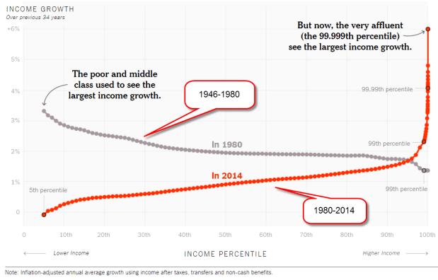
For several decades, Thomas Piketty and Emmanuel Saez have collected the aggregate income and tax data of developed countries. Piketty is the author of Capital in the Twenty-First Century (Capital), which I reviewed here.  A recent NY Times article referenced a report from Piketty and Saez comparing the growth of after-tax, inflation-adjusted incomes from 1946-1980 (gray line labeled 1980) and 1980-2014 (red line labeled 2014). I’ve marked up their graph a bit.
IncomeGrowth1947-2014
The authors calculated net incomes after taxes and transfers to determine the effect of tax and social policies on income distribution. Transfers include social welfare programs like Social Security, TANF, and unemployment. Census Bureau surveys of household income include pre-tax income and it is these surveys which form the basis for the calculation of the GINI index and other statistical measures of inequality.

I am guessing that Piketty and Saez used their database of IRS post-tax income data then adjusted for transfer income based on Census Bureau surveys. The Census Bureau notes that people underreport their incomes on these surveys.  Is the IRS data more reliable?  Probably, but people do hide income from the IRS. Both Piketty and the Census Bureau note that the data does not capture non-cash benefits like food stamps, housing subsidies, etc.

From 1947 to the early 1960s, the very rich paid income tax rates of 90% so that would seem to explain the after-tax income data from Piketty and Saez. The federal government took a lot of money from the very rich, paid off war debts, built highways, flew to the moon and built a big defense network to fight the Cold War.  Those infrastructure projects employed the working class at a wage that lifted them into the middle class. So that should be the end of the story. High taxes on the rich led to more equality of after-tax income.

But that doesn’t explain the pre-tax income data from the Census Bureau. The very rich simply made less money or they learned how to hide it because of the extremely high tax rates.  In the Bahamas and Caymans, there grew a powerful financial industry devoted to hiding income and wealth from the taxman. In the first years of his administration, President Kennedy, a Democrat, understood that the extremely high tax rates were hurting investment, incentives and economic growth.  He proposed lowering both individual and corporate rates but could not get his proposal through the Congress before he died.  Johnson did push it through a few months after Kennedy’s death. The rate on the top incomes fell from 91% to 70%, still rather high by today’s standards.

An important component of income growth in the post war period from 1947-1970 was the lack of competition from other developed countries who had to rebuild their industries following World War 2. These two decades were the first when the government began collecting a lot of data, and this unusual period then became the base for many political arguments. Liberal politicians like Bernie Sanders and Elizabeth Warren advocate policies that they promise will return us to the trends of that period. It is unlikely that any policies, no matter how dramatic, could accomplish that because the rest of the world is no longer recovering from a World War.

We could enact a network of social support policies that resemble those in Europe but could we get used to a 10% unemployment rate that is customary in France? For thirty years beginning in the early 1980s, even Germany, the powerhouse of the Eurozone, had an unemployment rate that exceeded 8%. At that rate, many Americans think the economy is broken. Despite 17 quarters of growth, unemployment in the Eurozone is still 9.1%. Half of unemployed workers in the Eurozone have been unemployed for more than a year. In America, that rate of long term unemployed is only 13% (WSJ paywall).

The post-war period was marked by high tax rates and high federal spending, a period of robust government fiscal policy.  The federal government intervenes in the economy via a second channel – the monetary policy conducted by the central bank.  The Federal Reserve lowers and raises interest rates, and adjusts the effective money supply by the purchase or sale of Treasury debt.

The 1940s, 1970s and 2000s were periods of high intervention in both fiscal and monetary policy. The FDR, Truman, Eisenhower, Johnson and Nixon administrations exerted much pressure on the Fed to help finance war campaigns and the Cold War. In 1977, the Congress ensured more independence to the Federal Reserve by setting two, and only two, clear objectives that were to guide the Fed’s monetary policy in the future: healthy employment and stable inflation.

A rough guide to the level of central bank intervention is the interest rate set by the Fed. When rates are less than inflation, the Fed is probably doing too much in response to some acute or protracted crisis.

EffFundsRate-Infation

Let’s look at an odd – or not – coincidence. I’ll turn to the total return from stocks to understand the effects of central bank policies. There are two components to total return: 1) price appreciation, and 2) dividends. When price appreciation is more than 50% of total return, economic growth and company profits are doing well. Future profit growth looks good and more money comes into the market and drives up prices. When dividends account for more than half of total return, as it did in the 1940s and 1970s, both GDP and company profit growth are weak. Both decades were marked by heavy central bank and government intervention in the economy.

Here’s a link to an article showing the total return on stocks by decade. During the 2000s, the total return from stocks was below zero. An average annual return of 1.5% from dividends could not offset an annual loss of 2.4% in price appreciation. Hubris and political pressure following 9-11 led Fed Chairman Alan Greenspan to make several ill-advised interest-rate moves in the early 2000s that helped fuel the housing boom and the ensuing financial crisis. His successor, Ben Bernanke, continued the policy of heavy intervention. Following the financial crisis, the Fed kept interest rates near zero for nine years and has only recently begun a program of gradually increasing its key interest rate.

The price gains of the 2010s have lifted the average annual return of the past 18 years to 7.4%, and the portion from dividends is exactly half of that, at 3.72% per year.  It has taken extraordinary monetary policy to rescue investors, to achieve balanced returns  that are about average from our stock investments.  Some investors are betting that the Fed will always come to the rescue of asset prices.  That same gamble pushed the country to the financial crisis when the government did not rescue Lehman Brothers in September 2008.

The financial crisis should have been on each generation’s list.  Within ten years it will be.  It is still crouched in the tall grass.

///////////////////////////

Debt

Happy days are here again.  Yes, girls and boys, it’s time to raise the debt ceiling!  By the end of September, the Treasury will run out of money to pay bills unless the debt ceiling is raised. This past week, President Trump hinted/threatened that he would not sign a debt increase bill unless it included money to build the wall between the U.S. and Mexico.

The Congress has not had a budget agreement in several years and is unlikely to enact one this year. People may sound tough on debt but a Pew Research study
showed that a majority do not want to cut government programs, including Medicaid.

Liberal economists insist that government debt levels don’t matter if the interest on the debt can be paid. This article from Pew Research shows the historically low rate on the federal debt. However, Moody’s reports that the U.S. government pays the highest interest as a percentage of revenue among developed countries. As a percent of GDP, we are 4th at 2.5%.

The Eclipse of Optimism

August 20, 2017

We are coming up on an anniversary of sorts. Two years ago, the stock market had a series of sell offs in the last week of August. China devalued the yuan, commodity prices around the world swooned, and Greece was in imminent default on its loans. Pictures of empty cities in China prompted speculation that the building boom in China was coming to an end and would bring down the global economy. Over the course of 6 days, the SP500 shed 11%.

By year’s end the SP500 was still slightly below its level at the end of August and did not rise above its mid-2015 price till the summer of 2016. Long term assets at the end of 2015 declined slightly for the first time since the financial crisis (ICI 316 page pdf). There wasn’t a rush for the exits but clearly some investors were spooked. Should I get spooked when the next 10% drop comes?

In the past five years there were 73 daily declines of more than 2% in the SP500 index.  That’s more than one in twenty trading days or about one per month.  2% is more than 400 points on the Dow at current levels.  One bad day per month was relatively mild compared to the previous five-year period from August 2007 to August 2012. Bad days with greater than 2% declines occurred more than once a week!

I wondered if a bad week telegraphed a long term severe decline in stock market prices. Let’s say that within five trading days, the stock market fell 10%, averaging more than a 2% decline on each of those five days. I started my search twenty years ago and each bad week had its own story.

The list:
the LTCM financial crisis of October 1998,
the end of the dot com boom in April 2000,
the week following the attack on 9-11,
the bankruptcy of giant WorldCom and other accounting scandals in July 2002,
the winter months of 2008-2009 during the financial crisis,
the budget battle and fears of the U.S. government defaulting on its debt in August 2011, and the devaluation of the Chinese yuan in August 2015.

In each case investors were jolted by a surprise or some ongoing concern deepened into despair and a rush for safety. In some cases, the crisis ended or a solution was found and the dip was a good buying opportunity. In other cases, the fears signaled a severe and sustained repricing as in 2000–2003 and in 2008-2009.

Let’s say I interpreted a 10% dip as a good time to increase my equities. Imagine the sinking in my belly when stocks continued falling another 20, 30, or 40% as in the two repricing periods above. How could I have been so stupid?

Just as losses of 10% in a week are not reliable predictors of doom, gains of 10% in a week are inconsistent predictors of a market recovery. When bad weeks happen, financial pundits seem so sure that a 50% drop in the market is imminent. The data shows that this is not the case.

Now I’ll turn up the dial and see if I can find any consistency. A drop of 15% in a week is rare. In sixty years, the only instances of this are in October 1987, and October and November of 2008. In each case, there was more pain to come after that initial fall. So, if I happen to be alive when the next 15% weekly drop comes, the market has probably not finished correcting. The only 15% gain in a week was in November 2008, following an almost 20% fall the previous week. Boy, those were the good old days – not.

Since historical data does not give a clear guide for short to mid-term outcomes, my best strategy in reaction to a bout of market darkness may be – gulp! – do nothing. That can be so difficult when I am bombarded with forecasts of catastrophe at those times.  The sun will shine again.  It’s only an eclipse.

Wage Growth – Not

August 12, 2017

Ratios are important in baseball, finance and cooking, in economics, chemistry and physics, and yes, even love. If I love her a lot and she kinda likes me a little, that’s not a good ratio. I learned that in fourth grade.

Each week I usually turn to one or more ratios to help me understand some behavior. This week I’ll look at a ratio to help explain a trend that is puzzling economists. The unemployment rate is low. The law of supply and demand states that when there is more demand than a supply for something, the price of that something will increase. Clearly there is more demand for labor than the supply. I would expect to see that wage growth, the price of labor, would be strong. It’s not. Why not?

I’ll take a look at an unemployment ratio. There are several rates of unemployment and there is no “real” rate of unemployment, as some non-economists might argue at the Thanksgiving dinner table. The rates vary by the types of people who are counted as un-employed or under-employed. The headline rate that the Bureau of Labor Statistics (BLS) publishes each month is the narrowest rate and is called the U-3 rate. It counts only those unemployed people who have actively searched for work in the past month. In the same monthly labor report, the BLS publishes several wider measures of unemployment, U-4 and U-5, that include unemployed people who have actively searched for a job in the past 12 months. U-6 is the widest measure of unemployment because it includes people who are under-employed, those who want full-time work but can only find part-time jobs. Included in this category would be a person working 32 hours a week who wants but can’t find a 40 hour per week job.

The ratio that helps me understand the underlying trends in the labor market is the ratio of this widest measure of unemployment to the narrowest measure. This is the ratio of U-6/U-3. In the chart below, this ratio remained in a narrow range for 15 years. Unemployment levels grew or shrank in tandem for each group. By 2013, the ratio touched new heights, climbing above 1.9 then crossing 2 in 2014. The two groups were diverging. The U-3 rate, the denominator in the ratio, was improving much quicker than the U-6 rate that included involuntary part-time workers.

U-6-U-3Ratio

What would it take to bring this ratio down to 1.85? About 1.5 million fewer involuntary part time workers. What does that involve? Let’s say that those involuntary part-time workers would like an average of 15 more hours per week of work. That is more than 20 million more hours of work per week, which seems like a lot but is less than a half percent of the approximately 6.1 billion hours worked per week in the 2nd quarter of 2017.  These tiny percentages play a significant role in how an economy feels to the average person.

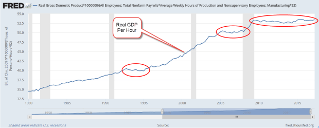
Let’s turn to a ratio I’ve used before – GDP per hour worked. I don’t expect this to be a precise measurement but it reveals long term trends in productivity. In the chart below, GDP per hour has flatlined since the end of the recession.

GDPPerHour201706

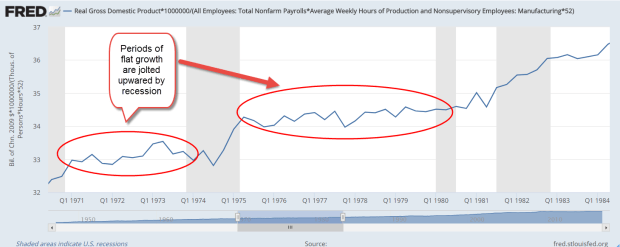
There are two ways to increase GDP per hour: 1) productivity gains, or more GDP per hour worked, and 2) reduce the number of hours worked more than the reduction in GDP. Door #1 is good growth. Door #2 is the what happens during recessions. GDP per hour rises because hours are severely reduced. I would prefer slow steady growth because the alternative is painful. Periods of no growth can be wrestled out of their torpor by a recession, a too common pattern. There were two consecutive periods of flat growth followed by recession in the 1970s and from the mid-2000s to the present day.

GDPPerHour1971-1984

The economy can withstand two years of flat growth without a recession as it did in the early 1990s. It is the long periods of flat growth that are most worrisome. In the early 1970s and late 2000s, the lack of growth lasted three years and were followed by hard recessions. The lack of growth in the late 1970s led to the worst recession since the 1930s Depression. GDP per hour growth has been flat for eight years now and I am afraid that the correction may be hard as well. Maybe it will be different this time. I hope so.

///////////////////

Participation Rate

Some commentators have noted the relatively low Civilian Labor Force Participation Rate (CLFPR). This is the number of people who are working or looking for work divided by the population aged 16 and older. (BLS). The rate reached a high of 67% in 2000 and has declined since then. For the past few years, the rate has stabilized at just under 63%.

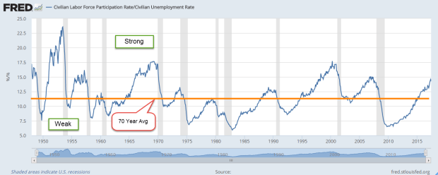
A graph of the rate doesn’t give me a lot of information. Starting in the 1960s, the rate rose slowly as more women came into the workforce and the large boomer generation came into their prime working years. So I divide that rate by the unemployment rate to look for long term cyclic trends. Notice that this ratio peaks then begins a downward slide as recessions take hold.

CLFPR-UI1947-2017

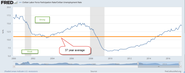
In mid-2014 this ratio finally broke above a long term baseline average and has been rising since. Today’s readings are nearly at the peak levels of early 2007.

CLFPR-UI

Some pundits use the CLFPR as a harbinger of doom that includes: 1) too many people are depending on government benefits and don’t want to work; 2) there is a shrinking pool of workers to pay for all these benefit programs; 3) thus, the moral and economic character of the nation is crumbling. During the 1950s and 1960s, when the participation rate was lower than today, our parent’s generation managed to pay off the huge debts incurred by World War 2. It is true that benefit programs were much less than those of today.

In “Men Without Work” Nick Eberstadt documents a long term decline in the percentage of prime age (25 – 54) males who are working.  Some interesting notes on shifting demographics: foreign born men of prime working age are more likely to be working or looking for work than U.S. born males. According to the Census Bureau’s time use surveys, less than 5% of non-working men are taking care of children.

In 2004 the participation rate for white prime age males first fell below those of prime age Hispanic males and has remained below since then.  In 1979, 10% of black males aged 30-34 were in jail.  In 2009, the percentage was 25%.

So why should I care about participation rates and wage growth? Policies initiated in the 1930s and 1960s instituted a system of inter-generational transfer programs.  In simple terms, younger generations provide for their elders. Current Social Security and Medicare benefits are paid in whole or in part by current taxes. We are bound together in a social compact that is not protected by an ironclad law.  Beneficiaries are not guaranteed payments.

For 40 years, from 1975-2008, the number of workers per beneficiary remained steady at about 3.3 (SSA fact sheet). In 2008, the financial crisis and the retirement of the first wave of the Boomer generation marked the beginning of a decline in this ratio to the current level of 2.7.

In their annual reports, both the SSA and the Congressional Budget Office note the swiftly changing ratio.  Within twelve years, the ratio is projected to be about 2.3.  In 2010, benefits paid first exceeded taxes collected and, in 2016, the gap had grown to 7% (CBO report) and will continue to get larger.

Policy makers should be alert to changes in the participation rates of various age and ethnic groups because the social contract is built partly on those participation rates.  As with so many trends, the causes are diffuse and not easily identifiable.  Economic and policy factors play a part.  Cultural trends may contribute to the problem as well.

Congress has a well-established record of not acting until there is an emergency, a habit they are unlikely to change.  Fixing blame wins more votes than finding solutions, but  I’m sure it will all work out somehow, won’t it?


Storage Costs

August 6th, 2017

Last week I discussed the concepts of present and future money. This week I’ll look at the costs involved in storing our money for future use. When I store my fishing boat over the winter, I pay storage costs. When I store money for the future I also pay storage costs. Some of these costs are outright fees. If I have a financial advisor, I may pay them a percentage based on the amount of money they manage for me. All mutual funds charge a fee which is clearly stated in the fund’s prospectus. Pension funds charge fees as well and that is not always as clearly stated.

In addition to fees, there are implied costs. My bank lowers the interest rate they pay me for savings and CD accounts to take care of their operating costs and profits. I could put my future money under my pillow but inflation eats away at my store of future money like rats in a granary bin.

Let’s turn to another cost that is more of a packaging cost– income taxes. But wait, taxes come out of my present money, my income. How can that be a cost of my future money? In the progressive income system that we have in this country, my income is taxed. If I make more money than my neighbor, I will pay a higher rate. My neighbor may pay an effective tax rate of 5% and I pay 15%.

We pay taxes on our leftover income – what we could put away into our store of future money. Let’s say that the median household income is $50K and my family makes $70K. The difference is $20K more than the median. It’s money that I could put into my store of future money. On the other hand, my neighbor’s household makes $40K, or $10K less than the median. Part of my family’s income that I could have put away for the future is going to be taken by the government in taxes.  Some of it will be used as a fee to pay for today’s common expenses like defense, police and courts, research, and infrastructure. Part of it will be given to my neighbor as a transfer payment. My future money becomes my neighbor’s present money.

How did I get my present money, my income? Invariably, it came from someone else’s future money which was previously saved and invested in a business that either hired me or contracted with me. All this money is on a merry go round of time.

Now let’s turn to the prospects for my future money. This article lists 22 reasons for not investing more money in equities at current valuations. I have mentioned several points covered in this article. One is the percentage of household wealth that is invested in the stock market. This past month, that percentage surpassed the level at the peak of the housing boom in 2006-2007.

StocksPctFinAssets201706

Maybe this time is different but I won’t count on it. The heady peaks of the dot-com boom in the late 1990s shows that this can go on for some time before the whoosh! comes.

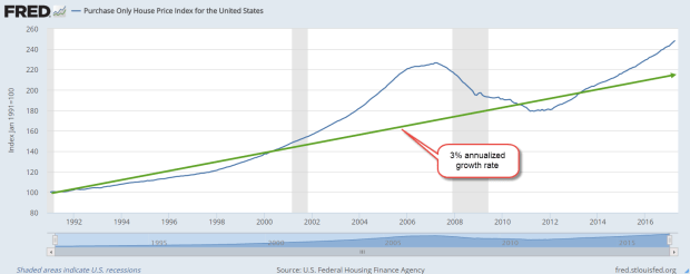
Housing prices continue to grow above a sustainable trend line. I’ve marked out a 3% annualized growth rate on the chart below. This housing index is for home purchases only and does not reflect refinances.

PurchaseOnlyHPI201706

Check out the growth in commercial real estate loans.  The 10% annual growth of 2015 and 2016 has cooled somewhat in the first two quarters of 2017 but is still a torrid 7.6%.  (Source)

CommlRELoans

Several years ago, I thought that real estate pricing would not get frothy again for several decades. We had all learned our lesson, hadn’t we? Maybe I was wrong. The worth of an asset is what the next buyer will pay for it.  Zillow tells me I am growing richer by the day but there’s a problem.  If I did sell my home, what would I buy?  Everywhere I look, housing prices are so expensive.  Now I come back full circle to another storage cost – storing the future me.