Find the Hidden Value

September 25, 2022

by Stephen Stofka

This week the SP500 index closed down more than 20% from its closing price at the beginning of the year. Where did the value go? When stocks were rising where did the value come from? Trained in neoclassical economics, the economist John Maynard Keynes asked the same question. He criticized the conventional economic analysis because it focused only on the present, disregarding the flow of money and goods into and out of the marketplace. Let’s explore that flow this week.

Let’s imagine that there is a car company called Drive whose stock symbol is DRV. When its stock price goes down on Monday, there were more sellers than buyers. The quantity of shares has not changed but the market value has declined. Where did that value go?

Let’s say that Sally bought 100 shares of DRV for $40,000 cash, or simply $40. I’ll leave off the 1000s in this story. She could have spent the money on a new SUV – satisfying her current needs – but buys a stock which she hopes will someday be used to satisfy her future needs. A car dealer did not make a sale. Let’s assume that the dealer has $36,000 cost invested in the vehicle.

What did the stock seller do with the proceeds? We might trace the money through many transactions in the stock market but eventually we come to Sam who took the proceeds from the sale of his 100 shares of DRV and bought a Drive SUV for $40. Sam’s net cash position is $0. A measure of economic activity, Final Sales of Domestic Product (BEA, 2022), has increased by $40,000 .

To recap the beginning positions: Sally = $40 cash, Sam = $40 stock, Drive dealer = $36 invested in car. Total = $116K. Let’s leave out income taxes, sales taxes and brokerage fees to keep the story simple.

A month later, the price of DRV goes down so that the market value of a 100 shares of stock is $36. The value of Sam’s SUV is not affected – or is it? If Sally were to sell her newly acquired shares at the lower price, she could buy a less expensive car but not that brand of SUV. Thus, there is less demand and the market for SUVs is softer because of the decline in DRV’s stock price.

Let’s imagine that Sally and Sam meet at the grocery store. Sally likes the SUV and offers to sell her DRV stock to Sam for $36, the market value. Sam thinks that is a good deal. He now has the same quantity of shares that he had before. If he had held onto the stock, the market price of the stock would have gone down anyway. He has driven the SUV for 1000 miles for free except for the gasoline. The dealer has $36 cash, covering the cost of the SUV, and $4 in cash profit.

Let’s recap: Sally = $36 car, Sam = $36 stock, Drive dealer = $40 cash. Total = $112K.

Sam and Sally each have $4,000 less than they started with for a total of $8,000 less. The dealer has $4,000 more than they started with. Where is the other $4000? Is it in the SUV’s depreciation or the stock’s lower market value?

/////////////////////

Photo by HAMZA YOUNAS on Unsplash

BEA: U.S. Bureau of Economic Analysis, Final Sales of Domestic Product [FINSAL], retrieved from FRED, Federal Reserve Bank of St. Louis; https://fred.stlouisfed.org/series/FINSAL, September 22, 2022.

Inflation and Profit Flow

September 18, 2022

by Stephen Stofka

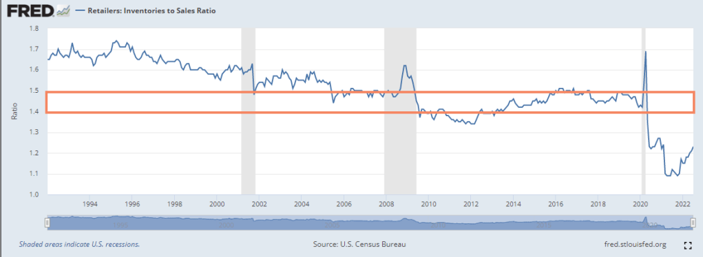
Price records circumstances, not value or utility. Our buying power is like a bar of soap. As water shrinks soap, high inflation shrinks our buying power. Economists offer several explanations for the persistent inflation but the one that I buy is that constrained supply and fairly steady demand are driving prices higher. Rising prices are a symptom of a shortage of goods – a quantity issue. Retailers inventory to sales ratio has increased slightly from the historic low in May 2021 but the ratio is still far below the range of 1.4 – 1.5 that was the benchmark before the pandemic.

This past Thursday, I picked up three jars of my favorite crunchy peanut butter. Some stores have been out of stock on the crunchy variety so I bought extra to be sure. I was not concerned about rising prices. I was responding to a quantity shortage, or the fear of a shortage. The difference is important. In Econ 101, students are shown the standard supply and demand diagram.

Left out of this stylized relationship is that supply is on a slower time scale than demand. It takes time, planning, investment and risk to produce all that supply. To cope with that reality, businesses must keep an inventory on hand to meet changes in demand which happen on a shorter time scale. Shift the red supply line to the left and the intersection of supply and demand occurs at a higher price. The Fed and the market thought that the supply constraints would fully resolve by this year but they have not. As stores and restaurants reopened, customers put away the electric panini sandwich makers, bread machines and gym equipment they had bought during the pandemic. They began purchasing consumables and were willing to pay higher prices for clothes, airline and movie tickets, and restaurant meals. In the face of ongoing supply constraints, the Fed has had to keep raising interest rates to try to curb demand, shifting the blue demand line to the left as well.

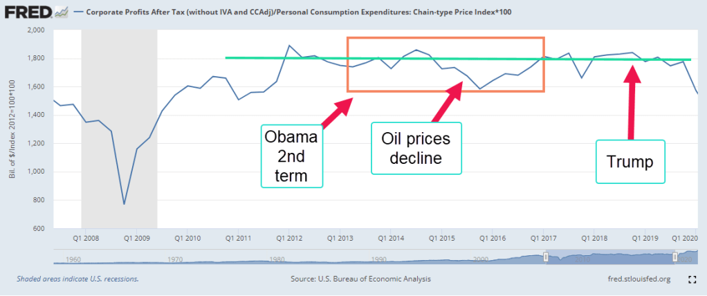
The higher prices helped businesses recover profits lost during the pandemic. Businesses have taken advantage of the supply disruptions to juice their profits by 33% (BEA, 2022).

When the Republicans took control of both chambers of Congress and the Presidency, they lowered corporate taxes. Those on the left often blame the economic elite for society’s problems and wasted no opportunity in criticizing Republicans for gifting the corporate elite. Mr. Trump boasted on his business prowess, promising to get the economy revving up again. Despite his rhetoric, corporate profits remained at the same level as during Mr. Obama’s second term.

A Presidential veto can block legislation but it is Congress that passes the laws that affect the economy. As I wrote last week Congress sometimes buys voter approval, creating bubbles that finally implode. The State Historical Society of Iowa (2019) has an image of a 1928 campaign ad for Herbert Hoover. It is a resume of economic progress under total Republican control during the 1920s. The Congress had won the public’s approval with easy credit and lax regulation. The following year the onset of the Great Depression brought down the house of cards. 25% of workers lost their jobs. Many lost their homes and farms.

Corporations exist to turn money flows into profits. Whatever money Congress spends winds up in corporate coffers. After 9-11, the federal public debt rose by $3 trillion (U.S. Treasury Dept, 2019) while corporate profits more than doubled, all thanks to Congress. Democrats and Republicans supported higher military spending and a building boom supported by easy credit policies.

In response to the pandemic, a bipartisan effort in Congress passed relief packages of more than $3 trillion. Today the public debt is $7 trillion above the pre-pandemic level. Much of that money became corporate profit because that’s what good companies do – turn cash flows into profits. Some of those profits were then used to buy the Treasury bills generated when the government increased their debt. This completed the cycle of debt and profits.

On average voters re-elect 90% of House members and 80% of Senate members. Midterm elections are less than two months away. Both parties take advantage of the public’s tendency to pin responsibility – good or bad – on the President, both the current and the past President, Mr. Trump. “Inflation is Biden’s fault,” Republicans will say and hope it sticks with some voters. Democrats hope that Trump will announce a 2024 run for President before the coming midterm election. They hope that independent voters, particularly suburban women, will vote for Democrats to voice their disaffection with Mr. Trump.

The election spending will juice the profits of media companies who depend on the craziness of our democratic politics. People in western European countries look in dismay at our frenzied politics that makes us vulnerable to a populist like Trump. Some Americans long for authoritarian measures that might curb the craziness of our politics and promote more cooperation. They are tired of the demolition derby of American democracy and wish they could go to sleep for a few months until it is over.

////////////////////

Photo by Anvesh Uppunuthula on Unsplash

State Historical Society of Iowa. (2019, January 14). “A chicken for every pot” political ad, October 30, 1928. IDCA. Retrieved September 16, 2022, from https://iowaculture.gov/history/education/educator-resources/primary-source-sets/great-depression-and-herbert-hoover/chicken If you have a moment, do check this out!

BEA: U.S. Bureau of Economic Analysis, Corporate Profits After Tax (without IVA and CCAdj) [CP], retrieved from FRED, Federal Reserve Bank of St. Louis; https://fred.stlouisfed.org/series/CP, September 16, 2022.

U.S. Department of the Treasury. Fiscal Service, Federal Debt: Total Public Debt [GFDEBTN], retrieved from FRED, Federal Reserve Bank of St. Louis; https://fred.stlouisfed.org/series/GFDEBTN, September 16, 2022.

America 4.0

September 11, 2022

by Stephen Stofka

I hope that those in the UK can find some common ground in their grief over the Queen’s death this week. Britain was still recovering from World War 2 when the crown was laid on her young head in 1952. Seventy years later, the political culture has fractured over Brexit and the repercussions of leaving the EU. There is much needed investment in a nation that has barely managed 2% growth in the past decade. In three years, three Prime Ministers have led the Parliament. The long reach of the Queen’s lifetime can help us lift our heads and take a longer view of events. When we mark history in lifetimes, not years, the beginning of our nation was about three lifetimes ago.

For most of mankind’s history, production harnessed human or animal energy, the thermal energy stored in wood and coal, and the kinetic energy of falling water turning a mill. In a world with only gradual change, there was little need for rapid communications technology. The men – yes, all men of property and standing – who crafted and voted on the U.S. Constitution lived in a world limited by crude animal and chemical power for energy, transportation and communication. John Adams, one of the Constitution’s signers, spent weeks traveling from his wife, family and farm in Braintree, Massachusetts to Philadelphia, Pennsylvania. Today, a person on a bicycle can make the journey in three 10-hour days.

The discovery and refinement of oil as an energy source changed our society and our politics. The 13th, 14th and 15th amendments of the Reconstruction Era were ratified at the dawn of a new age of energy and communications. The telegraph had only just come into use just prior to the Civil War. Edwin Drake drilled the first oil well in Pennsylvania in 1859, two years before the start of the Civil War. Those who passed the initial ten amendments and made the amendment process so difficult lived in an era where transformations of society occurred over decades or centuries. The amendments meant to protect people from the yoke of a regal government now shackle us to a historical reality that no longer exists.

America was built on a lack of consensus between regions, between a newly emerging urban population in the north and a rural population harnessed to the land in the south. In 1776, the colonies had first cohered as a mutual defense pact against the  British and the encroachment of the Spanish and French on colonial territory. The seven year war of Independence liberated the colonies from British rule in 1783 but left the colonies with a large debt. Their mutual defense pact gave a lot of autonomy to each of the thirteen states but the central government had little power or authority to tax the individual states. By 1787, that confederacy was on the brink of failure, unable to pay its debts and largely isolated from international capital markets. Under those dire circumstances, the colonies ed anew, drafting an entirely different pact that initiated America 2.0.

The American Constitution embodied the divisions of regional interests and the differing ideological principles of its founders. The proceedings were so combative that the deliberations were sealed from the press for fear that exposing the rancor between delegates would doom the  process. Three lifetimes later, we exhibit the same level of discord as our founders. Our Senate has become an insipid institution, crippled by parliamentary rules that make any Senator the ruler of his own nation, the King of Negation that stops most legislation from reaching a vote in the chamber. For 25 years, the House has passed Continuing Resolutions (CR) because they cannot pass a budget on time (Wezerek, 2018). Some years the budget is never passed and the government operates under a year-long CR.

On this 21st anniversary of 9-11, we still live in its shadow. The precautions at the airport, the fastidious matching of our names, letter for letter, hyphen for hyphen in our identification. Our nation grieved together, our Congress stood together and passed the Patriot Act. That was the end of togetherness. A common grieving does not knit a nation for long. Our media speaks a common language but the discourse – the assumptions and values that form the bedrock of our perceptions – are so different. Why? Because our Constitution has died.

Distrustful of each other, the Constitutional delegates forged a pact that was difficult to amend. They bound it so tightly that it could not expand and breathe. It is like a dead Pharoah mummified in tightly wrapped cloth and buried deep within a pyramid of time. Each year, the justices of the Supreme Court venture into the tomb to ask questions of the dead Pharoah. When they emerge into the sunlight, the people gather round to hear what the dead Pharoah has revealed. The justices speak in tongues – discourses that are intelligible to some people and babble to others. The Civil War was America 3.0. Let us grieve that our Constitution has died and adopt a new pact to celebrate America 4.0.

/////////////////////

Photo by Jeremy Bezanger on Unsplash

Wezerek, G. (2018, February 7). 20 years of Congress’s budget procrastination, in one chart. FiveThirtyEight. Retrieved September 9, 2022, from https://fivethirtyeight.com/features/20-years-of-congresss-budget-procrastination-in-one-chart/

Labor Trends

September 4, 2022

by Stephen Stofka

On this Labor Day Weekend I’ll review some current employment numbers and look at a historic trend whose results surprised me. The August employment report released this past Friday buoyed the stock market. Job gains remained strong but moderated from the half million jobs gained in July. The slowing gains indicated a predicted response to rising interest rates. Had the number of job gains risen to 600,000 for example, the market might have sold off. Why? Currently the market is predicting a rise in rates to a range of 3.5 – 4.0% in the next year. A labor market resistant to rising rates would have implied that the Fed would have to set rates even higher to cool inflation. Secondly, the unemployment rate rose .2% to 3.7%, another indication that rising rates are having a modest effect on employment. Modest is the key word.

The participation rate – the percentage of working age people who are working or looking for work – rose slightly to 62.4%, still 1% below pre-pandemic levels. Reopening classrooms and the further relaxing of pandemic restrictions are contributing factors. Additional family members may be joining the workforce to cope with rising household expenses. The number of marginally attached workers – those who want a job but haven’t actively looked for a job in the past month – declined to 5.5 million, still a half million above pre-pandemic levels. These “discouraged” workers remain below 1% of the labor force, a level indicating a strong labor market. President Obama inherited an economy in crisis and the percent of discouraged workers declined to nearly 1% but not below. As the rate fell below 1% in the first months of the Trump presidency, Mr. Trump cheerfully took credit. A politician and his followers blow their horns to encourage others others to join their coalition.

Surprises

A 17,000 employment gain in financial jobs surprised me. Rising interest rates have lowered mortgage applications and I thought the employment numbers for the financial industry would decline. Lastly, weekly earnings are up over 5.6% but have not kept up with inflation. Unemployment numbers are low, job openings are high. Why don’t workers have more pricing power?

A Historic View

Earlier this week I was looking at labor slumps since World War 2. These slumps are periods at least six months long. They start when the number of workers first declines. They end when employment finally surpasses its previous high. Employment first declines about two months after the start of a recession, as the NBER later determines it*, so it is a lagging indicator.

I split the period 1950-2022 into two 36 year periods. The first period lasted from 1950-1986; the second period from 1986-2022. In the first period there were 7 recessions and employment slumps. In the second period there were 4 recessions and slumps. Even though there were more recessions in the first period, the number of months of sagging employment was far less than the second period, 131 vs 168. No doubt that was due to the 75 month long slump of the Great Recession. That’s an extra three years of a lackluster job market which affected demand for workers and the pay they could command. In the chart below I have sketched the labor slumps. Economic recessions have a lasting impact on the labor market.

In the first period, the longest slump lasted 26 months during the early 1980s recession when the unemployment rate rose above 10% and inflation was in the teens. That began in September 1981 and lasted until November 1983. In the second period, the job market sagged during the Great Recession for 75 months, from February 2008 until May 2014. The least severe slump was this last one, beginning in April 2020 and ending in April 2022. The recession in 2001 lasted only 6 months but the labor slump lasted 40 months, from June 2001 until October 2004, just before the 2004 election.

Wages

More prolonged slumps affect wages. In the chart below the BLS compares nominal and inflation-adjusted median weekly earnings over the past twenty years. The real earnings of workers have barely risen because they are not sharing in the productivity gains of the past decades. The earnings gap between men and women has varied little during that time.

Contributing Factors

Why are labor slumps lasting longer during this later period? There are many contributing factors. When there was a larger manufacturing base recessions were more frequent but workers were brought back to work more quickly. The two recessions of the 2000s made that decade the hardest on workers. The two labor slumps totaled more than five years during the decade.

The 1970s gets a bad rap but it was the 1950s which had the second largest number of months when employment sagged – a total of 3.5 years. Standing five decades apart, the 2000s and 1950s had very different economic and family structures. Fewer women worked in that post war decade. The waiting period for unemployment insurance was twice as long and benefits lasted less than four months. These were inducements for workers to find any kind of work to support their families. Union membership was much higher in the 1950s so workers could rely on those benefits while unemployed. They would not have wanted to lose their union membership so they might have worked off the books for cash while they waited for hiring to pick up at the same company or the same industry. Like so many economic trends, the interaction between factors is complex and not readily identifiable.

Conclusion

Reckless speculation was the main contributor to the two recessions in the 2000s. Financial shenanigans played a smaller role in the slump of the early 1990s. The increased length of these slumps in the last four decades supports an argument that our economy has lost too much of its manufacturing base and is out of balance. There is too much financial speculation and not enough actual production. The federal deficit has increased so much in the past two decades because the private economy cannot generate enough growth on its own.

//////////////

Photo by Patrick Schneider on Unsplash

*The NBER marks only the decline portion of a general economic slump so the gray shaded areas will be shorter than the labor slump. However, the chart illustrates the prolonged effect that an economic decline has on the labor market.

BLS. (2022). Median usual weekly earnings of full-time wage and salary workers by sex. U.S. Bureau of Labor Statistics. Retrieved September 2, 2022, from https://www.bls.gov/charts/usual-weekly-earnings/usual-weekly-earnings-over-time-total-men-women.htm

Price, D. N. (1985, October). Unemployment insurance, then and now, 1935–85. Social Security Administration. Retrieved September 3, 2022, from https://www.ssa.gov/policy/docs/ssb/v48n10/v48n10p22.pdf