A Broader Inclusion

November 27, 2022

by Stephen Stofka

Hope everyone had a good Thanksgiving. This week’s letter is about a type of income that we don’t often think about, how that affects asset values and a proposal to increase homeownership. With left over buying power, people purchase assets in the hope that the buying power of the asset grows faster than inflation. There are two types of assets: those that produce future consumption flows and collectibles whose resale value increases because they are unique, desired and in limited supply. An example of the first type is a house. An example of the second type is a painting. Let’s look at the first type.

House Equals Future Shelter

A house is a present embodiment of current and future shelter. The value of that utility depends on environmental factors like schools, crime, parks, access to recreation, shopping and entertainment. These affect a home’s value and are outside a homeowner’s control. A school district’s rating in 2042 may be quite different than its current rating. Our capitalist system and U.S. tax law favors home ownership in several ways. The monthly shelter utility that a home provides is capitalized into the value of a property. Every consumption requires an income, what economists call an imputed rental income. Two thirds of homes are owned by the person living there (Schnabel, 2022) and a little more than half are mortgage free. Unlike reinvested capital gains in a mutual fund, this imputed income is not taxed to the homeowner. Let me give an example.

If the market rate for renting a similar home were $2000 a month, that is an implicit income to the homeowner. Because there is no state or federal tax on that income, the gross amount of that $2000 would be about $2400. That’s almost $30,000 a year. After monthly costs for taxes, insurance and maintenance, the annual implicit operating income of the property might be $25,000. At a cap rate of 5% (to make the math easy), the capital value of the property is $500,000. Each year, Congress requires the U.S. Treasury to estimate the various tax expenditures like these where Congress excludes certain income items from taxes. The implied income on owning a home is called “imputed rental income” and in 2021 the Treasury (2022) estimated that the income tax not collected was $131 billion. How much is that? A third of the $392 billion paid in interest on the public debt. If we did have to pay taxes on that imputed income, it would lower the value of our homes. For many decades, Congress has not dared to include that implied income.

Mutual Fund Capital Gains

Let’s return to the subject of reinvested capital gains in a taxable mutual fund held outside of an IRA or pension type account. Some of what I am about to say involves tax liability so I will state at the outset that one should consult a tax professional before making any personal buy and sell decisions. When some part of a fund’s holdings are sold, a capital gain is realized from the sale and paid to the investor who owns the mutual fund. If the investor has elected to have dividends and capital gains reinvested, the money is automatically used to repurchase more shares of the mutual fund. The balance of the account may change little but there is a taxable event that has to be included in income when the investor completes their taxes for the year. Many mutual fund holdings recognize capital gains in December.

Mutual fund companies provide the tax basis or unrealized gain/loss for each fund but often do not include that information on the statement. The unrealized gain is the price appreciation has not been taxed yet. For example, the dollar value of a fund may be $50,000 and the unrealized gain $5,000. This is more typical of a managed fund than an index fund which does not adjust its portfolio as frequently as a managed fund. If an investor were to sell the fund to raise cash, they would pay taxes on the $5,000, not the $50,000. The unrealized gain in an index fund might by 70% of the value of the fund. If the fund value is $50,000, the unrealized gain could be $35,000 and the investor would owe taxes on that amount. An investor can minimize their tax liability with a judicious choice of which fund to sell. Again, consult a tax professional for your personal situation.

Affordable Homeownership

Let’s visit an imaginary world where people do not have to pay property taxes outright. Each year they can elect to sell a portion of their property to the city or other taxing authority. Cities sometimes place tax liens on properties when a tax is not paid. This would be like a voluntary lien making the city a temporary part owner of the property until the homeowner sells it.

Imagine that a homeowner owns a home worth $400,000. For ten years, they have elected to have the city deduct an annual $2000 average property tax from the value of the home. Over the ten year period, the accrued sum is $20,000 plus an interest fee that is added to the principal sum of the tax. These voluntary tax liens would be visible to a lending institution so that the sum would lower the home’s value for a HELOC, or second mortgage. The city would report that annual amount each year as an imputed income to the homeowner and the homeowner would have to pay income taxes on it. At a 20% effective federal and state tax rate, the out-of-pocket expense would be about $480 on $2000. After the 2017 tax law TCJA, property taxes are no longer deductible so the homeowner has to earn $2400 to pay the $2000 tax outright. There is a slight change in income tax revenue to the various levels of government. When a home is sold those tax liens would be paid back to the city.

Why don’t we have such a system in place now? In the U.S. private entities own most of the capital. Some people would be uncomfortable knowing that a government authority had some legal claim to their property but they could opt out. In a pre-computer age, the accounting would have been a nightmare. Such a system is feasible today. Mutual fund companies have demonstrated that they can track the complex capital positions of their customers. Cities can do the same.

Such a system would make home ownership more affordable for a lot of people without affecting those homeowners who preferred to pay the property tax outright as we do under the current system. Investment companies would be eager to amortize those voluntary tax liens held by city governments. In the event of another financial crisis, a decline in housing prices and a rise in foreclosures, the city would be first lienholder, first in line to get paid when the property is foreclosed. Interest groups that advocate for affordable housing would be joined with investment and pension companies who wanted to underwrite the bonds for such a program.

A Capitalist System of Greater Inclusion

Some blame our capitalist system for the inequities in our society. The fault lies in us, not the capitalist system. Feudalism, mercantilism, capitalism, socialism, communism and fascism are systems of rules that embody a relationship of individuals to 1) property and the manner of production, both current and future, 2) the society, our families and communities, 3) the government that recognizes those relationships. The capitalist system is the most versatile ever invented and yes, it has been used to exclude people just as the other systems have been used to weaken some classes of people. The capitalist system can be extended to include and strengthen more of us. This homeownership policy could broaden that inclusion.  

////////////////

Photo by Hannah Busing on Unsplash

Schnabel, R. (2022, August 19). Homeownership facts and statistics 2022. Bankrate. Retrieved November 24, 2022, from https://www.bankrate.com/insurance/homeowners-insurance/home-ownership-statistics/

U.S. Treasury . (2022, October 13). Tax expenditures. U.S. Department of the Treasury. Retrieved November 24, 2022, from https://home.treasury.gov/policy-issues/tax-policy/tax-expenditures. Click FY2022 for the current year PDF estimates.

Profits and Savings Diverge

November 20, 2022

by Stephen Stofka

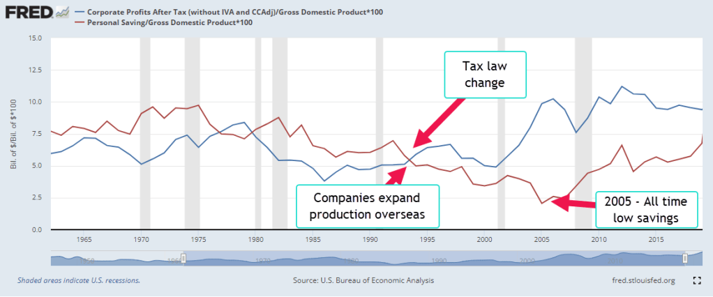
This week’s letter is about household savings and corporate profits. As a share of GDP, savings are near an all-time low while profits are at an all-time high. Elon Musk, the CEO of Tesla, appeared in court this week. No, this wasn’t about his acquisition of Twitter. It concerned a shareholder lawsuit against Tesla regarding the $50B stock option package the company awarded him in 2018. In 2019 the company’s total revenue – not profit – was less than $25B. In 2022, annual revenue was $75B. At a 15% profit margin, the company must continue growing its revenue at a blistering pace to afford Mr. Musk’s incentive pay package. Large compensation packages like this are only a few decades old. Let’s get in our time machine.

In 1994, Kurt Cobain, the 27 year old leader of the rock group Nirvana, died from an overdose of heroin. Something else was dying that year – corporations were breaking free of national boundaries and moving production to countries other than their home nation. This was the last stage in the evolution of multinational corporations, or MNCs. In earlier decades, companies had licensed or franchised their brand. Perhaps they had set up a sales office in a foreign country. Now they were becoming truly global. Fueling that expansion was an increase in equity ownership by large institutional investors. To accommodate these changes, their governance structures changed. Executives capable of leading this global growth were rewarded on a parallel with superstar sports talent. That was the conclusion of Hall and Liebman (2000, 3), two researchers at the National Bureau of Economic Research. 

Let’s look at two series over the past sixty years – personal savings and corporate profits. If we think of a household as a small enterprise, personal savings is the residual left over from the household’s labor. Likewise, corporate profits are the residual left over from current production. In 1994, the two series diverged. Corporate profits (the blue line in the graph below) kept rising while personal savings plateaued for a decade. Each series is a percent of GDP to demonstrate the trend more easily.

Executive Compensation

In the mid-1990s, corporations began to issue a lot more stock options to their executives. Some think that a change in the tax code might have precipitated this shift in compensation.  In 1994, Section 162m of the IRS code limited the corporate deductibility of executive pay to $1 million (McLoughlin & Aizen, 2018). By awarding non-qualified stock options to their executives, companies could preserve the corporate tax deduction. However, the slight tax advantage did not account for the rapid increase in options awards. Hall and Liebman found that the median executive received no stock option package in 1985. By 1994, most did. The tax change was secondary – a distraction. Institutional investors wanted more growth and more profits and companies were willing to reward executives with compensation packages similar to sports stars (Hall & Liebman, 2000, 5). Some of these superstars included Jack Welch of General Electric,  Bill Gates of Microsoft, Michael Armstrong of AT&T.

Income Taxes – Less Savings

In 1993, Congress passed the Deficit Reduction Act that raised the top tax rate from 31% to almost 40%. Personal income tax receipts almost doubled from $545 billion in 1994 to almost $1 trillion in 2001. The booming stock market in the late 1990s produced big capital gains and taxes on those gains. For the first time in decades the federal government had a budget surplus. However, more taxes equals less personal savings so this contributed to the flatlining of personal savings during that period.

Household Debt Supports More Spending

During the 2000s, personal savings remained flat. On an inflation adjusted basis, they were falling. Too many people were tapping the rising equity in their home to pay expenses and economists warned that household debt to income ratios were too high. Savings as a percent of GDP fell to a post-WW2 low. As home prices faltered and job losses mounted in late 2007, people began to save more but their debt left them with little protection against the economic downturn. During 2008, personal savings began to increase for the first time in fifteen years. More savings meant less spending, furthering the economic malaise that began in late 2007.

Multi-National Corporate Profits

During those 15 years corporate profits rose steadily as companies increased their global presence. Beginning in 1994 U.S. companies began shifting production to Mexico where labor was cheaper. In 2001, China was admitted to the World Trade Organization (WTO) and production outsourcing continued to Asia. Despite the profit gains, companies kept their income taxes in check. In 2021, corporate income taxes were at about the same level as in 2004. That contributed to the rising budget deficit during the first two decades of this century.

Federal Deficit

The prolonged downturn in 2001-2003 and the financial crisis and recession of 2007-2009 put a lot of people out of work. This triggered what are called “automatic stabilizers,” unemployment insurance and social benefits like Medicaid, housing and food assistance. The federal government went into debt to pay for the Iraq War, pay benefits to people and help fill the budget gaps in state and local budgets. The tax cuts of 2003 enacted under a Republican trifecta* of government control reduced tax revenues, further increasing the deficit. During George Bush’s two terms, the debt almost doubled from $5.7 trillion to $11.1 trillion.

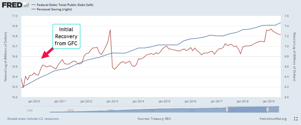
In coping with the recovery from the financial crisis, the government added another $8.7 trillion to the debt. That negative saving by the government helped add to the personal savings of households but too much was spent on just getting by. Following the Great Financial Crisis (GFC), the trend of the government’s rising debt (blue line below) matched the trend in personal savings (red). Sluggish growth and lower tax revenues caused the two to diverge. While the debt grew, personal savings lagged.  

Before and During the Pandemic

Following the 2017 tax cuts enacted under another Republican trifecta, personal saving rose, then spiked when the economy shut down during the pandemic and the federal government sent stimulus checks under the 2020 Cares Act. In the chart below, notice the spike in debt and savings. By the last quarter of 2020, personal savings had risen by $600 billion from their pre-pandemic level of $1.8 trillion. In late December, President Trump signed the $900 billion Consolidated Appropriations Act (Alpert, 2022) but that stimulus did not show up in personal savings until the first quarter of 2021. In March 2021 President Biden signed the $1.7 trillion American Rescue Plan. Personal savings rose $1.6 trillion in that first quarter, the result of both programs.

After the Pandemic

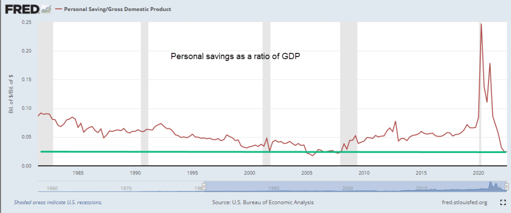
Some economists have said that the American Rescue Plan was too much. In hindsight, it may have been but we don’t make decisions in hindsight. As more schools and businesses opened up, households spent far more than any extra stimulus. They spent $1.2 trillion of savings they had accumulated before the pandemic and savings are now at the same level as the last quarter of 2008 when the financial crisis struck. Thirteen years of cautious savings behavior has vanished in a few years. On an inflation-adjusted basis, personal savings is at a crisis, almost as low as it was in 2005. In the chart below is personal savings as a ratio of GDP.

The Future

In the past year savings (red line) and corporate profits (blue line) have resumed the divergence that began almost three decades ago. Profits were 12% of GDP in the 2nd quarter of 2022. Savings is near that all time low of 2005. Rising profits benefit those of us who own stocks in our mutual funds and retirement plans. However, the divergence between the profit share and the savings share is a sign that the gap between the haves and the have-nots will grow larger.

////////////////////

Photo by Jens Lelie on Unsplash

  • A trifecta is when one party controls the Presidency and both chambers of Congress.

Alpert, G. (2022, September 15). U.S. covid-19 stimulus and relief. Investopedia. Retrieved November 19, 2022, from https://www.investopedia.com/government-stimulus-efforts-to-fight-the-covid-19-crisis-4799723. See Stimulus and Relief Package 4 for the December 2020 CAA stimulus. See Stimulus and Relief Package 5 for the American Rescue Plan in March 2021.

Hall, B. J., & Liebman, J. B. (2000, January). The Taxation of Executive Compensation – NBER. National Bureau of Economic Research. Retrieved November 19, 2022, from https://www.nber.org/system/files/chapters/c10845/c10845.pdf. Interested readers can see Moylan (2008) below for a short primer on the recording of options in the national accounts. Until 2005, these options were recorded as compensation for tax purposes but not recorded on financial statements so they did not initially affect stated company profits.

McLoughlin, J., & Aizen, R. (2018, September 26). IRS guidance on Section 162(M) tax reform. The Harvard Law School Forum on Corporate Governance. Retrieved November 18, 2022, from https://corpgov.law.harvard.edu/2018/09/26/irs-guidance-on-section-162m-tax-reform/

Moylan, C. E. (2008, February). Employee stock options and the National Economic Accounts. BEA Briefing. Retrieved November 19, 2022, from https://apps.bea.gov/scb/pdf/2008/02%20February/0208_stockoption.pdf

The Change Changed

November 13, 2022

by Stephen Stofka

October’s CPI report released this week indicated an annual inflation of 7.7%, down from the previous month. Investors took that as a sign that the economy is responding to higher interest rates. In the hope that the Fed can ease up on future rate increases, the market jumped 5.5% on Thursday. Last week I wrote about the change in the inflation rate. This week I’ll look at periods when the inflation rate of several key items abruptly reverses.

Food and energy purchases are fairly resistant to price changes. Economists at the Bureau of Labor Statistics (BLS) construct a separate “core” CPI index that includes only those spending categories that do respond to changing prices. It is odd that a core price index should exclude two categories, food and energy, that are core items of household budgets.

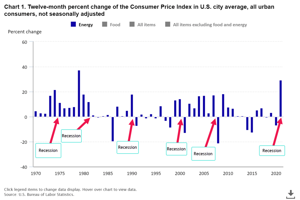
Ed Bennion and other researchers (2022) at the BLS just published an analysis of inflationary trends over several decades. Below is a chart of the annual change in energy prices. Except for the 1973-74 oil shock, a large change in energy prices led to a recession which caused a big negative change in energy prices.

We spend less of our income on food than we did decades ago so higher food prices have a more gradual effect, squeezing budgets tight. Lower income families really feel the bite because they spend a higher proportion of their income on food. In the graph below a series of high food price inflation often precedes a recession. Unlike energy prices, there is rarely a fall in food prices. Following the 2008 financial crisis, food prices fell ½% in 2009. It is an indication of the economic shock of that time.

Let me put up a chart of the headline CPI (blue line) that includes food and energy and the core inflation index (red line) which does not. Just once in 75 years, during the high inflation of the 1970s, the two indexes closely matched each other. Following the 1982-83 recession, the core CPI has outrun the headline CPI.

A big component of both measures of inflation is housing. The Federal Reserve (2022) publishes a series of home listing prices calculated per square foot using Realtor.com data. You can click on the name of a city and see its graph of square foot prices for the past year. You can select several cities, then click the “Add to Graph” button below the page title and FRED will load the graph for you. Here’s a comparison of Denver and Portland. They have similar costs.

The pandemic touched off a sharp rise in house prices in both cities. Denver residents have attributed the big change to an influx of people from other areas. However, Census Bureau data shows that the Denver metro area lost a few thousand people from July 2020 to July 2021 (Denver Gazette, 2022). In the decade after the financial crisis, there simply wasn’t enough housing built for the adults that were already here.

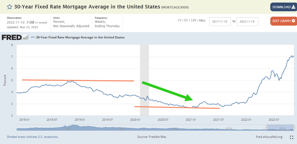
The surge in home buying has not been in population but in demographics. As people approach the age of 30, they become more interested in and capable of buying a home. The pandemic helped boost home buying because interest rates plunged from 5% in 2018 to 2.6% in 2021.

Record low interest rates enabled Millennials in their 20s and 30s to buy a lot more home with their mortgage payment. That leverage caused housing prices to rise. A 30-year mortgage of $320K has a monthly mortgage payment of $1349 at 3%. At 5%, it is $1718 and at 7% it rises to $2129. Ouch!

Rising rental costs and home prices drive lower income families to less expensive areas in a metro area or entirely out of an area. Declining public school enrollment has forced two Denver area counties to announce the closing of 26 schools and transfer them to other schools (Seaman, 2022). As the number of students decreases, the schools infrastructure costs do not change, increasing the per student costs. Buses have to be maintained, drivers paid, schools staffed with guards, cafeteria staff, janitors and administrative personnel. Once schools are shuttered, the building may be sold and converted to other uses, either residential or commercial. The public schooling system is like a large ship that takes some time to change course.

During our lifetimes we experience many changes. They can happen quickly or emerge over time. The effects may be short lived or last decades. Families are still living with the consequences of the financial crisis fourteen years ago. Carelessly planned urban development isolates the residents of a community. The social and economic effects can last several generations. As we grow older, we learn to appreciate William Faulkner’s line, “The past is never dead. It’s not even past.”

/////////////////////

Photo by Davies Designs Studio on Unsplash

Bennion, E., Bergqvist, T., Camp, K. M., Kowal, J., & Mead, D. (2022, October). Why inflation matters. U.S. Bureau of Labor Statistics. Retrieved November 11, 2022, from https://www.bls.gov/opub/btn/volume-11/exploring-price-increases-in-2021-and-previous-periods-of-inflation.htm

Denver Gazette. (2022, March 25). Denver joins big city trend with pandemic population slip. Denver Gazette. Retrieved November 11, 2022, from https://denvergazette.com/news/local/denver-joins-big-city-trend-with-pandemic-population-slip/article_65c6393d-2a4d-5b91-837c-f8c3efce3778.html

Federal Reserve. (2022). Median listing price per square feet:Metropolitan Areas. FRED. Retrieved November 11, 2022, from https://fred.stlouisfed.org/release/tables?eid=1138280&rid=462

Seaman, J. (2022, November 10). Schools targeted for closure in Denver, Jeffco have disproportionately high numbers of students of color, data shows. The Denver Post. Retrieved November 11, 2022, from https://www.denverpost.com/2022/11/10/dps-jeffco-school-closures-students-of-color/

////////////////////

Economic Puzzles

November 6, 2022

by Stephen Stofka

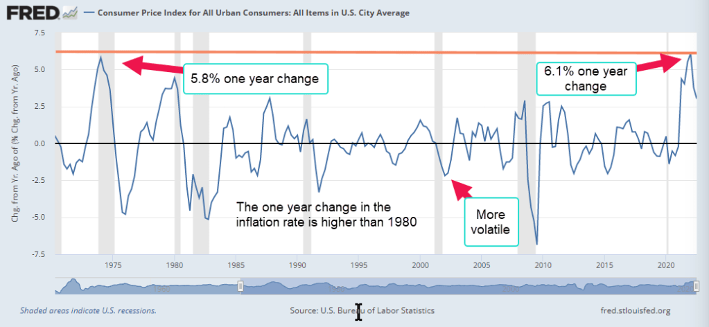
Many people compare today’s inflation with that of the 1970s. A better comparison might be with a much earlier period. This week’s letter will be about the change in the inflation rate. Inflation is like the speed on a speedometer. If I accelerated from 50 to 60 MPH over a certain time period, perhaps 10 seconds, the change in the speed is 10 MPH. The time period I’m looking at is one year. If inflation rose from 1% to 5% in a year’s time then the change is 4%.

I’ll start with the current year. The one year change peaked at 6.1% in the first quarter of 2022. As the Fed raised rates, that change moderated. It’s like accelerating to 60 MPH and realizing that the speed is over the speed limit and reducing speed by easing up on the gas pedal or braking.  

Most of the time the inflation rate changes by less than 2% up or down. During and after recessions it can become more volatile. In 1980, inflation soared above 14% and the one year change peaked at 5.8%, slightly less than our recent experience.

There has only been one time in the past 70 years when the inflation rate rose faster than today. That was in 1951, shortly after the Korean War began. For the first six months of 1950, prices sank – deflation – then war was declared in June 1950 and the U.S. again ramped up defense production. The one year change in inflation peaked above 10% as Federal defense spending shot up 45%.

If you would like to explore this period in more detail Tim McMahon (2014) presents 1950s inflation data in an easy to read format. A hundred years ago, a period of persistent deflation – not inflation – followed the last pandemic.  See Tim’s second link below. The Federal Reserve was still fairly new and the U.S. and European nations had adopted a gold standard that would eventually lead to the Great Depression. That’s another story. Today the world’s commerce is interlocked and pandemic shutdowns continue to deliver a series of supply shocks. Getting policy right is more difficult when circumstances are this unusual.

Volatile Inventories

Inflation rises when there are inadequate resources to meet demand. In 2021, real private gross domestic investment rebounded quickly, rising almost 32% on an annualized basis in the 4th quarter. One component, inventories, was responsible for much of that surge. Even under normal conditions, this series is a volatile component of GDP (BEA, 2019) and the BEA publishes a figure called Final Sales of Domestic Product which excludes the change in inventories. Real final sales is approximately close to inflation-adjusted GDP.

During the pandemic manufacturing and retail goods sat in container ships off the port of Los Angeles and other ports. While the goods were in transit, they were not added to inventories. In the 2nd quarter of 2021, businesses began to open again but the ports were slow to unravel their logjams. Empty truck containers sat in parking lots and on neighborhood streets near the L.A. port while ships waited in line out on the water.

Sales surged as economy reopened

In the 2nd quarter of 2021, real final sales increased 2%, finally reaching pre-pandemic levels. In the first half of the year, real food and service sales shot up 10%. Normally that increase would occur over three years. However, within months that initial surge subsided. Over the next two quarters, real final sales barely increased. Real food sales declined slightly. This confirmed a temporary response to a post-pandemic recovery. With so many items out of stock, customers were willing to pay higher prices to get products. Some businesses had orders shipped from Asia by air. In the 4th quarter 2021, the floodgates opened and real private inventories rose by a record $197 billion.

Profits Surge

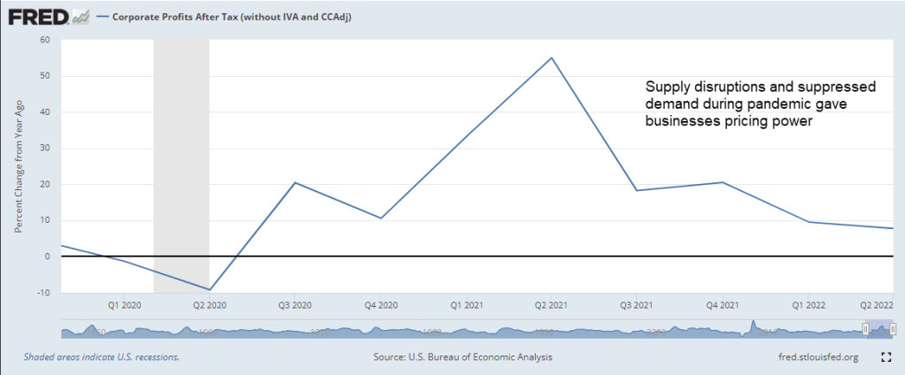
Real retail and food services sales fell slightly. In the last six months of 2021 inflation topped 5% but people were not buying and selling more stuff. Where were the price pressures? During the inflationary second half of the 1970s, profits increased a whopping 12% per year in those five years. In 2021, corporate profits rocketed up. Supply disruptions and repressed demand during the pandemic gave businesses pricing power. In 2021, corporate profits increased 18%. If demand was relatively flat, that pricing power had to fade but profit growth was still strong in the first quarter. Like the 1970s, rising corporate profits and pricing power were major contributors to inflation. This week the House Committee on Oversight and Reform (2022) came to a similar conclusion. What is the source of that pricing power?

War in Ukraine

In February 2022, Russia attacked Ukraine, sending energy prices higher. XLE, a broad energy ETF, gained 35% by early March. Two months later, the BEA reported another record rise in real private inventories of $214 billion. However, real final sales fell 2.5%. Some economists pointed to low unemployment and rising wages but ECI wages of private workers were on the same trend as before the pandemic when inflation was low. Most of the rise in the inflation rate was in housing, food and energy prices. The pandemic and low interest rates had contributed to the rise in housing costs. The war in Ukraine was responsible for volatile energy prices. There was no increase in real food sales but food prices were rising. Four large meat producers had profit growth of 134%, the committee reported.

The Puzzle

Historians still argue about the causes of World War I a century ago. Economists still cannot agree on the inflation mechanism of the 1970s. Contributing causes were rising corporate profits, shifting demographics in the work force, oil supply shocks, a shift in the international monetary regime and an evolving trans-global economy in the post war era. Economists do agree that it was a gestalt of market, fiscal and monetary forces, complicated by geopolitical and policy shocks that shaped expectations of future inflation. When people expect further price increases, they buy more now, aggravating inflationary pressures. Those expectations helped entrench inflation in the economy of the 1970s. Paul Volcker, chairman of the Fed in the late 1970s and early 1980s, raised interest rates so high that it wrung inflation out of the economy but at great economic cost to many families. The high interest rates caused two recessions, one of them the worst since the Great Depression.

The Korean War

In answer to the surge of inflation in 1951, the Fed raised rates slightly but rates stayed below 2%. The government did the heavy lifting. In September 1951, President Truman started a regime of wage and price controls administered by the Economic Stabilization Agency (ESA) and Wage Stabilization Board (WSB). There were loud protests against the controls and President Eisenhower ended them after he took office in 1953. Several months later the Korean War ended. In 1971, President Nixon instituted wage and price controls and demonstrated the failure of controls. Monetary policy is the weapon of choice to combat inflation but rising rates disproportionately affect the most vulnerable workers.

Conclusion

Infrequent events are an intersection of many factors that make each one unique. As economists pull apart the tangle of causal narratives, they develop new theories or modify existing ones. Economists usually cling to a favorite – either supply or demand. I’m watching profit growth. If Republicans take the House and possibly the Senate in the coming election, they will try to further enhance corporate profits at the expense of social programs like Medicare and Social Security. Republicans continue to sell a “trickle down” narrative but decades of evidence shows that the trickle is but a few drops. What goes to the top stays at the top.

///////////////////

Photo by Ana Municio on Unsplash

BEA: Bureau of Economic Analysis. (2019). Chapter 7: Change in private inventories. Retrieved November 4, 2022, from https://www.bea.gov/resources/methodologies/nipa-handbook/pdf/chapter-07.pdf

The House Committee on Oversight and Reform. (2022, November 4). Subcommittee analysis reveals excessive corporate price hikes have hurt consumers and fueled inflation, while enriching certain companies. House Committee on Oversight and Reform. Retrieved November 5, 2022, from https://oversight.house.gov/news/press-releases/subcommittee-analysis-reveals-excessive-corporate-price-hikes-have-hurt

McMahon, T. (2014, April 23). Inflation and CPI consumer price index 1950-1959. InflationData.com. Retrieved November 3, 2022, from https://inflationdata.com/articles/inflation-cpi-consumer-price-index-1950-1959/. Inflation data for 1920-1929 is here https://inflationdata.com/articles/inflation-consumer-price-index-decade-commentary/inflation-cpi-consumer-price-index-1920-1929/