Producer and Consumer Prices

February 4, 2024

by Stephen Stofka

This week’s letter is about the inflationary spurt that began a little over two years ago. The causes of the inflation have been a controversial topic among economists and political commentators. Some blame Biden and the Democrats for enacting a third round of stimulus shortly after he took office. That’s fiscal policy on the hot seat. Some target monetary policy, blaming the Fed for leaving interest rates at a pandemic low near 0%. In this letter, I will focus on a price signal that the Fed could have treated with more importance. A combination of the two is more credible. Republicans hope to make inflation and the immigration crisis at the southern border central issues in this year’s election campaign.

I’ll begin with two measures of changes in consumer prices. The Consumer Price Index, or CPI, is a headline gauge of inflation that reflects current price changes. Because Fed policy must anticipate price changes, it uses a  a less volatile index called the PCEPI, or Personal Consumption Expenditures Price Index. I’ll call it PCE. The CPI is based on a static basket of goods that the average family might buy each month. Households adapt to changing prices where they can but the CPI methodology does not measure that. Nor does it measure costs paid by someone other than the members of a household. To address those weaknesses, the PCE measures the actual spending choices that households make. The PCE includes expenses like health care benefits that an employer provides. The Cleveland branch of the Federal Reserve has a deeper dive on the differences between the two measures.

The oldest price index, first charted in 1902, is based on a measure of prices that producers and wholesalers receive at both the intermediate and final stages of production. In the final demand phase, a product is going to be sold to a consumer. In the intermediate stage a producer sells a product to another producer as a component in their product. Each month the BLS surveys thousands of companies to compile the wholesale prices on most of the goods sold in the U.S. and 70% of traded services. The agency then builds hundreds of indexes to measure the changes in those prices. The Producer Price Index, or PPI, is a headline composite of those indexes. As you can see in the graph below, the PPI is more volatile than the PCE measure of consumer price inflation. Government subsidies can increase the prices that suppliers receive with little impact on consumer prices. The PPI is more responsive to changes in transportation and distribution costs.

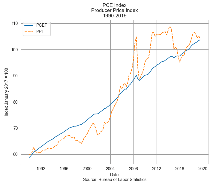
Despite its volatility, the PPI is regarded by the Fed, Congress and the administration as an advance indication of movements in consumer prices, according to the BLS. It indicates producers’ forecast of consumer demand and reflects economic stress and global supply pressures. However, wholesales prices may not be a reliable forecast tool of consumer inflation if the economy is weak and households cut back on their spending where they can. In the recovery years following the financial crisis in 2008, real GDP did not rise above 3% until the end of 2014. Unemployment finally dipped below 5% in the spring of 2016.

In 2021, the PPI indicated a developing surge in wholesale prices that would become apparent in consumer prices by the following year. But the economy still had not fully opened and unemployment did not fall below 5% until the fall of 2021. Would the pandemic recovery follow the sluggish trend of the recovery after the financial crisis? The Fed waited, preferring to keep interest rates low to support the labor market. In the graph below I’ve charted both the PCE and PPI over the past eight years. I’ve marked out the beginning of Biden’s term in the first quarter of 2021 and the Fed’s tightening that began in the spring of 2022.

The PPI (dotted orange line) had already reversed higher before Biden took office. As we can see in the chart above, the Fed did not enact stricter monetary policy until the PPI had peaked. In hindsight, the Fed was late to respond to surge in prices but Congress has given the Fed a dual mandate to maintain stable prices and full employment. During times of economic stress, those two objectives can indicate contradictory policies. During the initial months of the pandemic in 2020, five million people left the work force. In early 2020, the participation rate for the prime work force aged 25-54 stood at 83%. By the fourth quarter of 2021, the rate was still only 82%. 1.5 million workers had still not returned to the labor force. During a severe crisis like the pandemic, the Fed has trouble balancing those two objectives of stable prices and full employment. If they raised rates too soon, they could have damaged a recovery in the labor market.

While the general price level has come down in the past year, the inflation beast is not dead. There is still a residual inflation energy in some intermediate goods. Had the pre-pandemic price trends continued for the past four years, we might expect prices to be 8 to 10% higher than they were at the start of 2020. The prices of a number of goods have stabilized at levels far above their pre-pandemic levels. Meats are 32% higher after four years. Natural gas prices (WPU0551) have declined from the highs of last winter but are 38% higher than pre-pandemic prices. Residential electric power (WPU0541) and gasoline (WPU0571) are up 25% in four years. LPG gas is up 28% in that period. The prices of paper boxes (WPU095103) are up the same amount. Paper (WPU0913) is up 25%. The prices of bakery goods (WPU0211) are up 22% and still rising.

Despite promises made during the upcoming presidential campaign, the general price level is not going to return to its pre-pandemic level no matter who is president. The pandemic shook up the global economy, raised the general price level and there is no going back. A U.S. president may have their finger on the button of an arsenal of destruction but they have little influence on the producer prices of goods sold around the world. A hindsight analysis can identify policy winners and losers made by both the Trump and Biden administrations. The Fed and other central banks waited too long to respond to a worldwide inflation. Finally, the lessons learned from this pandemic will not all be applicable to the next global crisis.    

////////////////

Photo by Ian Taylor on Unsplash

Keywords: PCE, PPI, wholesale prices, consumer prices, inflation

Note: In April 2022 the Fed began raising its key interest rate by .25% or more each month.  

A Junk Drawer of Changes

December 8, 2019

A tip of the hat in respect to those servicemen who lost their lives at Pearl Harbor on December 7th, 1941 – almost 80 years ago.

This week I was cleaning out two kitchen drawers that had turned into junk drawers over the years. I became aware of how much things have changed in the past twenty years. There was a digital pedometer that we don’t use anymore. A cell phone app does that now. There were 9- volt batteries in the drawer that were long past their expiration date. The new lithium smoke and carbon monoxide detectors don’t need them. The manufacturer says to replace the entire unit after ten years. There were bayonet type Garden Accent light bulbs in the drawer. We use LED fixtures now. There were phone cords and phone couplers for landline phones. We don’t have those anymore. There were batteries for a modest digital camera. We use our cell phones to take photos now. There were expired C-batteries for a battery-operated adding machine that we don’t use anymore. Technology is changing more rapidly than I clean out my junk drawer. Maybe I should do that more often.

Talking about change….

I was in Amish country in Iowa a week ago. Although different communities have different rules, they ordinarily don’t use fossil fuels. We were in one store with a big iron wood burning stove. At a grocery warehouse, the clerk used a battery powered adding machine instead of a cash register. We saw a few men cleaning up the fields and tossing the remains of last season’s planting into a large container sized like a dump truck. It was pulled by a team of four horses. For tasks requiring gasoline, natural gas and electricity, the Amish rely on outsiders whom they call “English.” For farm work requiring a combine, they hire outsiders.

Most of us do not want to live the way of the Amish. We have become accustomed to the benefits of the very efficient energy provided by fossil fuels. Our society and economy thrive on energy. Stricter regulations have spurred technological advancements that enable our cars, furnaces and power plants to burn fuels much cleaner now. Climate scientists point out that we are putting far too much carbon dioxide in the atmosphere. Some scoff at the idea that carbon dioxide can be a problem. We breathe it out. Plants breathe it in. As part of the dynamic energy cycle, carbon dioxide itself is not a problem.

The threat to our way of life is the extra amount of carbon dioxide that our industrialized society is exhaling into our atmosphere. We are rapidly tapping a reservoir of carbon that was stored in the earth more than 300 million years ago. The key word in that sentence is “rapidly.” We are putting more carbon dioxide into the atmosphere than the plants can absorb. In some developing countries, people are cutting down the trees that absorb carbon dioxide as part of their life cycle.

From ice cores extracted from Greenland and the Antarctic climate scientists have been able to deduce a familiar cycle of events when the carbon dioxide concentration increases. The planet warms, the oceans rise, and precipitation increases. Permafrost at extreme latitudes melts and releases the carbon it has stored. That creates a feedback loop that intensifies the effect.

We need to slow down our consumption of fossil fuels, but we don’t want to give up the savings from the energy they provide. The internal combustion engine lowered food production costs, increased yields and lowered the cost of food for all Americans. Farmers dry their corn and other staple crops with fossil fuels. In another time, they might have plowed a damp surplus crop back into the ground.

We can’t attribute the lower cost of food entirely to fossil fuels, but a comparison of prices surprised me. A hundred years ago butter cost .58 per lb. in NYC (BLS, 2006). That’s $7.54 in current dollars. Eggs were .57 per dozen, so about $7.40. Current price for eggs was $1.28 last month (BLS, 2019). That’s a sixth of the price a century ago. Milk, a government subsidized product, was .28 per 1/2 gallon – approximately $3.64 in today’s money. The current price for milk is $3.12 for twice as much, a gallon. Milk today is about 40% of the cost it was a century ago.

Sixty years ago, the development of nuclear energy plants promised cleaner and less expensive energy. After the Three Mile Island accident in 1979, the building of new nuclear plants was severely curtailed [Wikipedia, n.d.]. Each year more coal miners die in accidents than all the people in history who have died from a nuclear accident. When it comes to nuclear, people disregard comparative statistics.

We don’t like making hard choices. We don’t like inconvenience. We absorb change and become accustomed to it. We put our old ways of doing things in the junk drawer of history and forget about it. We don’t want to live like the Amish to adapt to a planet with rising levels of carbon dioxide. What choices will future generations make?

/////////////////////////

Bureau of Labor Statistics (BLS). (2006, May). 100 Years of U.S. Consumer Spending. [Web page, PDF]. Retrieved from https://www.bls.gov/opub/100-years-of-u-s-consumer-spending.pdf

Bureau of Labor Statistics (BLS). (2019, November). Average Retail Food and Energy Prices, U.S. City Average and Northeast Region. [Web page, PDF]. Retrieved from https://www.bls.gov/regions/mid-atlantic/data/averageretailfoodandenergyprices_usandnortheast_table.htm

Photo by katherine cunningham on Unsplash

Wikipedia. (n.d.). Three Mile Island accident. [Web page]. Retrieved from https://en.wikipedia.org/wiki/Three_Mile_Island_accident#Effect_on_nuclear_power_industry

Budget Perspective

June 2, 2019

by Steve Stofka

How does your spending compare with others in your age group? Working age readers may compare their budgets with widely published averages that are misleading because they include seniors as well as those who are still living at home with their parents or are going to college. Let’s look at spending patterns classified by working age consumers 25-65 and seniors whose spending patterns change once they retire.

The Bureau of Labor Statistics collects data on consumer behavior by conducting regular surveys of household spending (Note #1). These surveys provide the underlying data for the computation of the CPI, the Consumer Price Index. Social Security checks and some labor contracts are indexed to this measure of inflation.

The BLS also provides an analysis of consumer purchasing by household characteristics, including age, race, education, type of family, and location (Note #2). Spending and income patterns by age contained some surprises (Note #3). The average income of 130,000 people surveyed in 2017 was $73K. Seniors averaged $25K in Social Security income. Younger workers aged 25-34, the mid-to-late Millennials, earned $69K, near the average of all who were surveyed. Following the Great Financial Crisis, this age group – what were then the early Millennials in 2010 – earned only $58K, so the growing economy has lifted incomes for this age group by 20% in seven years.

Home ownership is around 62% for the whole population, but far above that average for older consumers. 78-80% of people 55 and older own their own homes. More than 50% of those have no mortgage but too many seniors do not have enough savings. In many states, property taxes are the chief source of K-12 education funding and older consumers have the fewest children in school. Older consumers on fixed budgets resist higher property taxes to fund local schools and they vote in local elections at much higher rates than younger people. Since 2000, per pupil spending has grown more than 20% but most of that gain came in the 2000s.  In the past twelve years, real per pupil spending has barely increased (Note #4). Below is a chart from the Dept. of Education showing per pupil inflation adjusted spending.

Graph link: https://nces.ed.gov/fastfacts/display.asp?id=66

Saving is an expense and working age consumers aged 25-65 are saving 9-12% of their after-tax income, twice as much as the 5.6% average. Wait – isn’t saving the process of not spending money? How can it be an expense?  Call it the imaginary expense, as fundamental to our life cycle as i, the imaginary square root of -1, is to the mathematics of cyclic phenomena. Let’s compare today’s savings percentage with the panic years of 2009-10 just after the financial crisis. Workers in the 25-34 age group – who should have been spending money on furniture and cars and eating out – were saving 20% of their after-tax income (Note #5). That age group will probably carry the lessons – and caution – learned as they began their working career after the financial crisis.

Workers 25-65 spend 28-32% of their after-tax income on housing. Until they are 65, people spend a consistent 12% of their income on food, both at and away from home. Seniors spend less on food but most of that change is because they spend less money eating out at restaurants. Working age consumers spend more on transportation than they do on food – a consistent 15% of after-tax income.

People 65 and older are entitled to Medicare but they spend more on health insurance than working people and the dollar amount of their spending on health care rises by 50%. As a percent of after-tax income, seniors spend 15% while people of working age spend about 6%. Ouch. I’m sure many seniors are not prepared for those additional expenses.

Those of working age should compare their budget averages to other workers, not to the national averages, which include older people and those under 25. Summing up the major expense categories: workers are averaging 30% for housing, 15% for transportation, 12% for food, 11% for personal insurance, pensions and Social Security contributions, 10% for savings and 6% for healthcare.

As Joey on the hit TV show Friends would often say, “So how you doin’?”

///////////////////

Notes:

  1. Explanation of Consumer Expenditure Survey
  2. Consumption patterns – list Table 1300
  3. The most recent detailed analyses available are for 2017.
  4. Dept of Ed data
  5. Spending and income levels for those aged 25-34 2009-2010.

Housing and Stocks

February 23rd, 2014

The extreme cold in half of the country had a profound effect on housing starts which fell 16% in January.  Less affected by the weather are permits for new housing which slid 5%.

The Bible prescribes that every 50th year should be a Jubilee year, in which all debts are forgiven.  While this policy of redistribution of property might be a practical solution in a smaller tribal society, it is much less practical, even dangerous, in a complex economy.  By targeting a 2% inflation rate, central banks in the developed world engage in a type of gradual debt forgiveness.  Inflation incrementally shifts the real value of a debt from the debtor to the creditor.  At a 2% inflation rate, a debt is worth half as much in 35 years.

Let’s say Sam borrows $1000 from Jane at 0% interest and doesn’t pay her anything for 35 years, then pays off the debt.  The $1000 that Sam pays back in 35 years is only worth $500 in purchasing power.  Half of Sam’s debt has effectively been forgiven.  So why would Jane loan Sam any money?  She wouldn’t – not at 0% interest.  At that interest rate the loan is actually a gift.  Jane would need Sam to pay her an interest rate that 1) offsets the erosion of the purchasing power of the loan amount, the principal, and 2) compensates Jane for the use of her money over the 35 years.

Janes all over the world loan Sam the money and don’t want much interest.  The Sam in this case is Uncle Sam, the U.S. Government.  The loan is called a 30 year Treasury bond.  (Treasury FAQs )

If your name is just plain old Sam though, few people want to loan you money for thirty years, even if it is to buy a hard physical asset like a house.  That is why U.S. government agencies back most of the mortgages in the U.S., essentially funneling the money from around the world to ordinary Sams and Janes to buy housing.  Heck of a system, isn’t it?

The affordability of housing… 

In the metro Denver area, median household income was $59,230 in 2011, compared to the national median income of $50,054. (Source)  According to Zillow, the median home value in Denver is $253,700, or 4.3 times income.   Although Denver is a large city, it is not a megalopolis like New York City or Los Angeles. In Los Angeles, median home values are $491,000.  Median incomes in 2011 were $46,148, so that home values are more than ten times incomes.  Like other megaregions, Los Angeles has a huge disparity in housing and incomes, resulting in a median income that is skewed downward because of the large number of poor people that inhabit any large metropolitan area.  The L.A. Times ranks incomes by neighborhoods.  This ranking shows a median income in middle class areas at about $85K.  Using this metric, housing is still more than six times income.  Using a conventional bank ratio of .28 of mortgage payment to income, a household income of $85K will qualify for a monthly mortgage payment of almost $2K, which will get a 30 year, 4.5% fixed interest mortgage payment, including property taxes, of about $320K.  A 20% down payment of $80K brings the price of an affordable house to $400K, below the median value of $461K, meaning that many middle class Los Angelenos can not afford to live in a middle class neighborhood.

… acts as a constraint on home sales.
 

This week the National Assoc of Realtors reported a year over year 5% drop in existing home sales.  After rising more than 10% over the past year, prices have outrun increases in income.  While we don’t have median household income figures for 2013, disposable personal income actually declined in 2013 so we can guesstimate that household income was relatively flat as well.

As this year progresses, we may see other effects from the drop in disposable income.  Economists and market watchers will be focusing on auto and retail sales in the coming months.  January’s Consumer Price Index showed a yearly percent gain of 1.6%, indicating little inflationary headwinds.  An obstacle to growth is the difference between inflation and the weak growth in household income.

*********************************

Minimum Wage

On Tuesday, the Congressional Budget Office released their estimate of the net effect of raising the minimum wage to either $9 or $10.10 from the current Federal level of $7.25 an hour.  Their analysis ranged from a minimal loss of jobs to almost a million jobs lost.  The average of this range, 500,000 jobs lost, became the headline number.  The CBO also noted that over 16 million low income workers would see an increase in income, enabling some to rely less on government aid programs.  Their projection was a slight increase in revenues to government.  A half million jobs is relatively small in a workforce of 150 million.  Some economists would concur that there is no clear evidence that raising the minimum wage has any effect on the number of jobs.  The science of economics is the study of complex human behavior in response to changes in our environment and resources.  Many times the data is not as conclusive as one might like, leading researchers to statistically filter or interpret the data according to their professional biases.

A 2013 analysis of minimum wage workers by the Economic Policy Institute indicated that the average age of minimum wage workers was about 35 years old.  Yet, 2012 data from the Bureau of Labor Statistics, the primary aggregator of labor force characteristics, does not support EPI’s conclusions – unless one includes workers who are exempt from minimum wage laws – like waiters – who are paid below the minimum wage law.  The BLS data shows that 55% of minimum wage workers are below 25 years old.

Too frequently, financial reporters who could summarize the caveats of a particular study either don’t bother or their work is left on the editor’s floor.  Many readers digest the headline summary without question and a difficult guesstimate by a government agency like the CBO is re-quoted as though it were gospel truth.

**********************************

Manufacturing Rebound?
On the bright side, an early indicator of manufacturing activity in February showed a rebound from January’s decline.

********************************

Stock Market Dividends
As the market continues to rise, the voices of caution, if not doom, get louder.  Some analysts are permanent prophets of catastrophe.  Eventually they are right, the market sinks, they proclaim their skills of prognostication and sell more subscriptions to their newsletters.  Subscribers to these newsletters don’t seem to mind that the authors are wrong most of the time.

Last August, I wrote about the dividend yield – or it’s inverse ratio, the price dividend ratio – of the SP500 index using data that economist Robert Shiller compiles from a variety of sources.  The dividend yield of the SP500 index is currently 1.9%, meaning that for every $100 a person invested in the SP500 index, they could expect $1.90 in dividends.  The price dividend ratio is just the inverse of that, or $100 / $1.90 = 52.6. The current dividend yield is at the 20 year average.  I will focus on the dividend yield, or the interest rate that the SP500 index pays an investor.

It might surprise some investors that dividend information is available on a more timely basis than earnings.  In the aggregate,  dividends are more reliable and predictable.  Most companies have several versions of earnings and they massage their earnings to present the company in the best light.  On the other hand, most companies announce their dividend payouts near the end of each quarter so that the aggregate information is available to an investor more quickly than aggregate earnings.

Most portfolios contain a mixture of stocks and bonds so it is instructive to compare the dividend yield of the relatively risky SP500 with the yield on what is considered a perfectly safe bond – the 10 year Treasury.  Many investors think of these two asset classes as complementary – they are – but they are also in competition with each other. If the real dividend yield on stocks is the same as ten year Treasuries, it means investors in stocks want to be compensated for risking their principle on stocks.  If the interest rate on 10 year Treasuries is 4% and the  dividend yield of the SP500 is 2%, then the dividend ratio of stocks to Treasuries is 2% / 4%, or .5.  As investors perceive less risk in the stock market, this “demand for yield” from stocks will fall and the ratio will decline.   In the past, this ratio has reached a low of .19 in July 2000 as the stock market reached its apex of exuberance and investors became convinced that the rise of the internet and just in time inventory control had ushered in a new era in business.  Bill Gates, then CEO, Chairman  and founder of Microsoft, scoffed at dividends as a waste of money that could be better put to use by a company in growing the business. At the other extreme, this demand for yield ratio rose as high as 1.28 in March 2009 as stocks reached their lows of the recession.

More importantly is the movement of this ratio from peaks and troughs, indicating a change in sentiment among investors.  Note that the early 2003 market lows after the tech bubble burst were about the 50 year average of this ratio.  Compare that relative calm to the spikes of fear in this ratio since late 2007 to early 2008.  For the past 18 months, this demand for yield has declined but is still above the 50 year average.  There is still enough skepticism toward the stock market that it continues to curb exuberance.