Fortunate Son

November 10, 2024

By Stephen Stofka

The country has elected a fortunate son for the second time. Throughout his life, Donald has enjoyed the protection of a phalanx of lawyers who have kept him out of jail. A recent decision by the country’s highest court will give him immunity for another four years. His physical condition and cognitive health are declining so rapidly that he likely will not serve out his full term. His much younger Vice-President J.D. Vance will become President and possibly the leader of the MAGA movement for another eight years.

Another take. Former President Donald J. Trump has made the greatest political comeback in the history of this country. Millions of supporters donated money to his legal efforts to defend the integrity of the vote and challenge voter fraud by the Democratic Party. Despite persistent persecution by Democratic prosecutors, Mr. Trump has emerged victorious. In the days leading up to the election, the former President  held many rallies, demonstrating the vitality of a candidate twenty years younger.

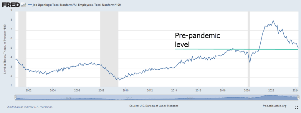
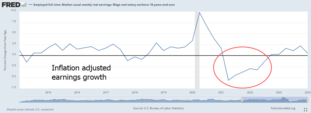
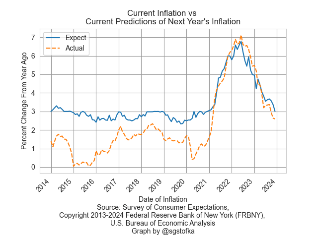
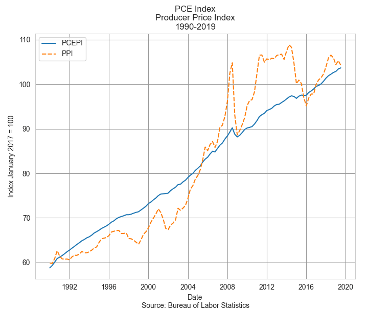
Yet another take – a just the facts, ma’am perspective. Presidents with low approval ratings, including Trump in 2020, do not win reelection. This election’s results repeated that trend. James Carville, Clinton’s campaign manager in the 1992 race, coined the famous phrase “It’s the economy, stupid.” Voters showed more concern about inflation and immigration than Trump’s character and demeanor. Voters are especially sensitive to inflation because they feel helpless, and people do not like feeling helpless.

The misery index is the sum of the unemployment rate and the inflation rate. A comfortable reading is about 7%. In 1980, the index was 20% and Jimmy Carter lost his bid for re-election. Bill Clinton and George W. Bush won re-election with misery readings of 8%, and Obama won the 2012 election when the misery index was near 10%. In the fall of this year, the index was below 7%. Perhaps the misery index is not a consistent predictor.

Which is your take on the election results? Each second of our day we download terabytes of information into our brains. We filter out much of that data, then arrange what remains into a version of the world that is uniquely ours. Then we interpret that stimuli, integrating it into our memories along well-worn neural pathways. In that integration process, we reconstruct the world again, discarding the information that conflicts with our previous experience, beliefs and values. We shape what we experience, and our experience shapes us. We may be traveling with others on a train through time, but we have a unique vantage point as we look out the window.

In her book Lost in Math, physicist Sabine Hossenfelder writes, “If a thousand people read a book, they read a thousand different books.” Each voter creates a unique election story. Media analysts focus on different elements of an election, creating their own version of the contest, weaving a narrative of cause and effect. In the telling of the election, we should remember Nassim Taleb’s caution, in Fooled by Randomness, that “past events will always look less random than they were.” Since we are rational creatures, we are both frightened and fooled by randomness. In an evenly divided electorate where a few thousand votes in several key counties can make a difference,  random events can decide the outcome. A snowstorm in a key state in the days before an election, the path of a bullet at an election rally, a decision by a federal judge.

The percentages of the Presidential election votes were no different than 140 million voters flipping a fair coin.. Heads equals a vote from Trump. Tails was a vote for Harris. Did any individual voter flip a coin? Possibly, but unlikely. As a collective, our individual actions can simulate random behavior. Randomness can make us feel helpless, so we act as though our actions have purpose. We act aggressively or assume a false bravado in the face of random mortal danger. Watch the clip from the Deer Hunter where the prisoners are made to play Russian Roulette.

Those who struggle through life may vote for the calm bravado of someone privileged. Ronald Reagan was known as the Teflon President. The public did not hold him responsible for several controversies and scandals that occurred during his eight years in the White House. In 1981 to 1982, the country suffered the worst recession since the Great Depression fifty years earlier. During the 1983 Lebanese civil war, Reagan ignored warnings that the U.S. Marines barrack in Beirut would be vulnerable to attack. The October 23rd bombing resulted in the loss of 241 lives, most of them Marines. . In his 1984 bid for re-election, Reagan won all but one state, a resounding vote of public approval. In 1986, the Iran-Contra scandal, a secretive trade of arms for hostages with Iran, occupied public attention but Reagan escaped any responsibility or public indignation.

Forty years later Donald Trump can wear that moniker, the Teflon President. A slim majority of voters overlooked his many scandals, his felony conviction, and his chaotic management style during the pandemic and most of his first term. Although the Republican Party’s name remains the same, Trump and his followers have erased the legacy of Reagan. The party’s former symbol, an elephant, has been replaced by a red MAGA hat. It has become a party dedicated not to any consistent set of principles but to one person, a fortunate son.

//////////////////

Photo by Danilo Batista on Unsplash

Keywords: misery index, election, recession, inflation

An Economic Nexus

September 8, 2024

by Stephen Stofka

This week’s letter is about the labor market, part of a series on investing. Friday’s monthly labor report indicated a job market that is cooling but still growing. Although the market reacted negatively to the news, the Fed will begin reducing interest rates at its meeting next week. The S&P 500 index, the most widely held basket of stocks, is up 15% for the year but the index has twice risen above 5500 before falling back. An index of business activity in the services sectors continues to expand but manufacturing activity is still contracting slightly. When investors get conflicting economic signals, they are responsive to negative data points more than positive ones. The approach of what may be a contentious election creates an environment where investors are more likely to protect their portfolio value and exit short-term positions. Let’s now turn to long-term trends in the labor market.

Economists at the Bureau of Labor Statistics (BLS) refer to workers aged 25 -54 as the core work force. To save some typing, I will refer to this age demographic as the “core.” During those thirty years we accumulate stuff while we build our careers. We buy cars, furniture, homes and vacations. We build retirement savings for ourselves and college funds for our kids. The core is the nexus of a growing economy.

This coming Wednesday we will remember 9-11 and the 3,000 civilian lives lost in the attack on the World Trade Center in lower Manhattan. Since that time, there has been little investment in those workers who form the core of the labor market. From August 2001 to August 2024, the economy has added less than seven million jobs in that age demographic, an annual growth rate of just 0.28% (See FRED Series LNS12000060).

As you can see in the chart above, most of the growth in the core has occurred during the Biden administration. The surge in employment in this age group led to growing incomes and greater purchasing power in an age group that is in the accumulation phase of its lifetime. That rapid growth in employment, coupled with pandemic recovery payments from the government were strong contributors to the rise in inflation in the 2021 – 2023 period. Voter sentiment in this age group focused on the inflation, not the job growth, demonstrating again that we pay more attention to negative rather than positive news.

Several factors contributed to the plateauing of job growth in the core. Demographics played some part. Population analysts have assigned a span of about 18 years to each generation so that the thirty-year span of the core labor force encompasses two and sometimes three generations. The first of the large post-war Boomer generation turned 54 in 2000. As the Boomers aged out of the core, a smaller Generation X, born 1964 to 1982, became the dominant component of this age group. In 2013, the first Millennials, a generation larger than the Boomers, joined the core, and in 2016, the last of the Boomers aged out of the core.

A few months after 9-11, China was admitted to the World Trade Organization, and within a decade became the world’s factory. Investors poured capital into China, taking advantage of low labor rates and a currency whose exchange rate was maintained at a low level by the Chinese central bank. Investors from outside China got more bank for their buck. As investment moved to China, many production facilities in the U.S. shuttered their doors. In the seven-year span between China’s admittance to the WTO and the start of the financial crisis in September 2008, manufacturing employment (see FRED Series MANEMP) fell by a fifth. By January 2010, employment in the manufacturing sector had declined by a third.

During the 2000s, low interest rates fed a frenzy in home financing and produced a bubble in the U.S. real estate market that imploded in 2008. The resulting financial crisis affected assets and financial institutions around the world. Millions of Americans lost their jobs. From the start of 2008 until the end of 2009, the core work force fell by 6%, about six million jobs. In 2018, an interval of ten years, the level of employment in this age group finally rose above its 2008 level.

Instead of vigorously promoting policies that encouraged job growth, the Obama administration offered policies to support families suffering from the lack of job growth. Democratic politicians eagerly passed ambitious social programs but faltered when implementing policy solutions that embodied their legislative goals. In Recoding America, Jennifer Pahlka (p. 125) recounts the efforts to fix healthcare.gov, the bungled rollout of the health exchanges created under the Affordable Care Act known as Obamacare. In The Rise and Fall of the Neoliberal Order, Gary Gerstle (p. 226) notes that the Obama administration focused more effort and political capital on providing healthcare insurance for poor people rather than supporting the 9 million households in danger of losing their homes to foreclosure.

A sense of betrayal soured voter sentiment and helped to support the emergence of the Tea Party in the 2010 election and the MAGA voters who supported Donald Trump’s candidacy in the 2016 election. In 1976, voters punished President Gerald Ford for pardoning Richard Nixon. In the 2016 election, voters punished Hillary Clinton as a symbol of a set of values disloyal to many Americans. Donald Trump promised to bring manufacturing jobs back to America by taxing Chinese imports and cutting corporate taxes. In the first three years after the 2008-2009 recession, manufacturing employment under Obama grew by more than it did in the first three years of the Trump presidency (see notes for details). No amount of political rhetoric can overcome the power of a supply chain now firmly anchored in Asia.

Biden’s infrastructure policies have actively promoted job growth in the core. Can the economy sustain such growth in this acquisitive age group while keeping inflation at a reasonable level? Should the Fed raises its target interest rate from 2% to 3% to accommodate job growth that supports people when they are raising families and building careers? I think so. Should Harris win November’s election, she should adopt Biden’s pro-growth policies. Should Trump regain office in the coming year, he will try to use tariffs to shift the nexus of the global supply network from Asia back to the U.S. That policy will only increase prices and help maintain a higher level of inflation without promoting the economic growth that supports households in their middle years.

 ///////////////

Photo by Tim Mossholder on Unsplash

Manufacturing employment notes: From January 2010 to December 2012 manufacturing gained 500,000 jobs, an increase of 4.4%. From January 2017 to December 2019, the manufacturing sector gained 432,000 jobs, an increase of 3.5%. In January 2010, manufacturing employment was near a low, continuing to fall after the official end of the recession in July 2009.

Keywords: Obamacare, inflation, labor, financial crisis, China, manufacturing, infrastructure

The Elasticity of Our Spirit

August 18, 2024

by Stephen Stofka

This week’s letter is about the effect of quantitative phenomena on our quality of life. Why do events impact people of the same socioeconomic circumstances differently? We are part of a group responding to the event, so we interact with the collective responses of the group around us. Our direct response to the event is a small part of the total impact on our quality of life. Imagine we are a rubber duckie in a group of rubber duckies on the ocean’s surface as a wave passes. As we rise with the water that displacement causes a lot of jostling by the duckies around us. Much of the effect we experience is not the wave but the reaction of the others around us to the wave. Yet we attribute the cause of our experience to the wave, not our fellow duckies.

One hundred years ago, Louis de Broglie introduced a wave theory of matter. A few years later Erwin Schrödinger proposed a wave equation of electron motion to explain the quantum world. Those two ideas are cornerstones of quantum mechanics, the most tested theory in physics and the foundation of our current electronic technology. As you read this on a computer or smart phone you are watching quantum mechanics at work. Not all wave are alike. Light and radio waves are electromagnetic waves that don’t need a medium to travel in. Even in the vacuum of space, the electromagnetic field they create acts as a type of medium. Some waves, called transverse waves, cause matter to move in a direction that is partly perpendicular to the force of a wave. A rubber duckie bobbing up and down in the water is an example.

We are hunters of cause. We are interested in the origin of phenomena, thinking that the origin of something will enhance our understanding of that thing. For that reason, some economists like to debate the origin of money. One morning a few weeks ago, our cat woke up, yawned and stretched out a paw on the bed. A claw caught in the quilt and slid it sideways so that it formed a tunnel. Like a wave through water, the direction of the paw was parallel to the quilt, but the quilt reacted in a direction perpendicular to that movement. Kitty pulled her paw back and the tunnel mostly collapsed. She then stretched out her paw again and the quilt rose up. Her hunter reasoning led her to believe that a mouse was the cause of the tunnel under the quilt, so she attacked. She pounced and pawed the quilt to find that imaginary mouse, then lost interest, jumped to the floor and left the room. How often do we search for the cause of a phenomena that is mostly a response to the collective action of a group?

When prices go up, we can look to our side for contributing factors, the decisions of many consumers and businesses. A quantitative change in prices affects the quality of our lives. Like a cat, we often judge quantitative phenomena with an instinctive appraisal. We notice the rise in prices more than we do the rise in our wages because we are more sensitive to loss than gains. The Bureau of Labor Statistics reports that the annual increase in average hourly wages and weekly earnings is now higher than inflation. A rise in the price of the goods we buy has a greater effect than a similar rise in our income because we perceive a rise in prices as a loss of our purchasing power. We are particularly loss averse, according to Daniel Kahneman, the author of Thinking Fast and Slow, who won a Nobel Prize for his research into the less than perfect reasoning we employ in our decision making. He and Amos Tversky proposed a concept called Prospect Theory to describe and model the mechanics of our decision making.

Elasticity is a term that economist John Marshall borrowed from physics to describe the reaction of consumers to changes in the prices of goods. The most common measure is called the Price Elasticity of Demand and businesses pay close attention to this metric. It is the change in the percentage of goods bought in response to a 1% change in price – a ratio of two percentage moves – the zig divided by the zag. If the price of butter goes up 1% and the amount of butter sold declines by 2%, then the ratio of percentages is 2 to 1 and butter is considered to be elastic. If the quantity of butter sold declines only 1%, then butter is said to be unit-elastic. If the quantity of butter barely changes, then it is inelastic. When businesses sense that consumer demand for their good or service is inelastic, they can charge higher prices with less effect on the quantity sold and make a higher profit. Businesses respond to consumer decisions and tastes.

The elasticity of economic goods is not constant because consumer demand responds to a changing economic environment, as well as tastes and culture. In some cases, consumer demand can change abruptly. Such was the case after the pandemic. The airline market is an example of two types of demand elasticities. Business travelers are much less sensitive to changes in price, with an elasticity far below 1, according to research done in the 2010s. Because of that airlines upcharge business customers. Leisure travelers, on the other hand,  have an elasticity of almost 2, meaning that they are sensitive to price hikes. The higher prices that airlines charge business customers effectively subsidizes leisure travelers. However, after the pandemic, the demand for leisure travel surged and airlines responded with higher prices. Average airline fares surged 20% annually in the summer of 2021 then rose sharply by 34% in the summer of 2022. In the first quarter of this year, prices stabilized to pre-pandemic levels. Vacation travel is a luxury good, but it can feel like a necessity when we feel stuck in a grind and stressed at work.

The effect is more frequent for necessities like food, lodging and utilities. That frequency affects the elasticity of our spirit the way a weight on a spring changes the spring’s elasticity over time. The relief checks sent during the pandemic helped some families build a small savings cushion, a relief from the burden of living paycheck to paycheck. In the past two years, families that have dipped into their savings to meet higher housing, grocery and childcare costs feel a sense of loss because their savings are smaller. Even if wage gains have kept up with inflation on average, wage gains are calculated based on gross income before taxes. We buy groceries and pay housing costs with after-tax dollars. The loss is real.

Like water, human society is the medium, transmitting and transmuting the force of thousands of decisions made by people we will never meet. Our circumstances and decisions affect the lives of strangers. There is no single cause because we are part of the cause. Even if we could identify a primary cause like rising prices and remove it with a magic wand, we cannot predict a satisfactory resolution. Yet politicians running for office hold out their magic policy wand and promise to end this or that problem, hoping that enough voters will buy what they are selling. “Here’s the problem,” they say. “I can do something about it.” We want to believe that complex processes have simple causes, and in the final months of this election year, candidates will tailor their message to our belief in that simplicity.

////////////// 

Photo by Joey Huang on Unsplash

Keywords: prices, inflation, cause, effect, wave

Key Expectations

June 9, 2024

by Stephen Stofka

This week’s letter continues my exploration of the role of expectations. They coordinate the supply, demand and price relationships that form the web of our economic and financial lives. They shape our voting patterns, and alter our behavior in interactions with others. If we expect a police officer to be hostile, we are defensive. That reaction will affect the behavior of the officer, increasing the chance that the encounter will be hostile. Expectations cause us to behave in ways that confirm and amplify our expectations, aggravating undesirable circumstances.

Expectations and yearnings act symbiotically within us but there is a distinction between the two. Expectations are a calculation; yearnings are a desire. “I think that” is an expectation. “I hope that” is a yearning. A woman may yearn to have a child, but she expects to have a child within a period of time. A yearning knows no time or logic. We expect a certain range of compensation for the type of work we do, our skill level and experience. Business coaches encourage people to visualize and enhance their good attributes to raise those expectations. Business owners expect their capital to earn a certain percentage of profit as compensation for the risk, planning and skill that a successful business requires.

Consumers expect a certain range of prices for many frequently bought goods and services. The price of meat may be more or less than average in a week, but the price will not be $100 a pound for ground beef. We may have no price anchor for infrequent purchases like replacing a hot water heater. A few hundred dollars or a few thousand? A search in a browser can help with an average price of approximately $2100 to help a homeowner evaluate quotes from a plumbing contractor.

In the U.S., the pricing of medical care is treated as a catastrophic event like a house fire. The connection between price and medical care has been cut so that patients may not know beforehand the price of a procedure. A browser search for the cost of a colonoscopy indicates an average cost of $2200, close to that of a hot water heater, coincidentally, but medical providers do not quote a price. Prices are negotiated between health insurance companies and a network of medical providers. The negotiated price may be a fifth of the stated list price. If patients have health insurance, the only price visible to them is a co-pay. The prospect of higher medical costs next year does not incentivize us to seek care now at a lower price. Colonoscopy prices going up soon? Let me book one now! However, as costs increase, workers negotiate for better benefit packages that cover the anticipated higher costs.

In our economy, workers play a dual role of producer and consumer. The monthly labor report and retail sales report captures the importance of these roles, and the release of these reports move markets. In the core labor force age range of 25 to 54, four out of five people are working or looking for work, according to the latest labor report. The largest generation in this demographic are the Millennials, born between 1981 and 1996. They produce the most and buy the most so their expectations steer the economy. Job openings as a percent of total employment indicate a historically robust labor market. Recent reports indicate that openings are returning to pre-pandemic levels.

Job openings as a percent of total non-farm employment

Despite the strong demand for labor, post-pandemic inflation has taken a bite out of gains in median earnings. Biden assumed office as earnings gains turned negative. Despite legislation meant to promote investment and support the labor market – the Inflation Reduction Act – the decline in real earnings did not turn positive until 2023.

Real earnings equals real purchasing power. Late Millennials reaching their early thirties expected to be able to settle down and buy a house. Older Millennials in their forties who expected to trade up to a different home are frustrated by high home prices and interest rates. Political power in our system is captured by the interests of older voters, particularly the Boomers. Less than one out of four in this generation is working (FRED series here). They want to reduce their tax costs, and preserve or enhance the government benefits they feel they have earned after a lifetime of working.

This week, David Leonhardt, editor of the N.Y. Times Morning Newsletter, pointed out a poll indicating strong support for many policies initiated by the Biden administration. Most of the public’s attention is directed to controversial issues like immigration, the war in Gaza and American support for Ukraine in their continuing war against Russia’s invasion. The pandemic focused the public’s attention on Trump’s chaotic governing style. His behavior defied expectations and his supporters became accustomed to excusing or rationalizing his actions. A majority voted for Biden as a return to normalcy in the recovery from the pandemic.

People vote their expectations, and those expectations strongly influence voters’ assessments of the economy even before a candidate has taken office. A candidate needs to offer a clear set of new expectations that manifest the yearnings of a majority of voters. Has either candidate made the connection between voter expectations and yearnings? Next week I will look more closely at the political aspect of expectations.

////////////////

Photo by Jan Tinneberg on Unsplash

Keywords: prices, growth, earnings, inflation

Invisible Expectations

June 2, 2024

by Stephen Stofka

This week’s letter continues a topic from last week, our expectations of inflation. The high inflation of the 1970s prompted a lot of debate on this topic, and I will try to cover a portion of those ideas. Hypotheses regarding the formation of expectations influence monetary policy and the manner in which the Fed raises interest rates. Different policy approaches reach across the country into the pocketbooks of many Americans. They can mean the loss of many jobs or few jobs, or the viability of buying a home.

The University of Michigan conducts a monthly survey of consumer sentiment in a rotating sample among 500 participants. Respondents are asked to estimate the rate of inflation for the next twelve months (see here, p. 5). Inflation is a rise in the average price of all goods but in casual conversation, we often use the term loosely to refer to a rise in prices of the goods and services that have the most impact on our lives. Each of our estimates are biased but an average of many estimates should approximate a comprehensive survey of the prices of many goods. This BBC five-minute video explains this phenomenon known as The Wisdom of the Crowd when many people try to estimate the number of jelly beans in a mason jar.

The blue line in the graph below is the headline CPI that tracks a basket of goods and excludes expenses like the employer portion of health care insurance. The Fed pays more attention to the PCEPI, the green line in the graph below. That methodology is based on actual expenditures in various sectors of the economy, including employer paid health insurance. Notice how closely the average estimates of inflation approximate this broad measure of price movement. In the April 2024 survey, expectations averaged 3.2%, a big decrease from over 5% in 2022 but a slight rise from 2.9% in March.

How do we form inflation expectations? There are two hypotheses, and they are distinguished by how errors occur in our expectations. Adaptive expectations was a predominant hypothesis until the 1970s. It holds that we revise our forecasts up when actual inflation is higher than we expected, and down when inflation data indicates that our forecast was too high (Blanchard, 2017). Imagine that we are offered a discount at the doctor’s office if we guess our weight within three pounds. We base our guess on a previous weight reading. If it is too low, we lose our discount so the next time we revise our guess higher. Under this hypothesis, our expectations are very much guided by past experience and our forecast errors are systemic. To tame high inflation, monetary policy must act like a shock that induces a recession and alters the expectations of investors and consumers.

In August 1979, during the Carter administration, Paul Volker assumed the position of Fed chair. In October, the Fed raised interest rates 1.5%, then lowered by a half-percent in November, then raised them again by a half-percent in December. In those three months, sales of new one-family homes (HSN1F) dropped 25%. A few months later, in the spring of 1980, came another interest rate shock of a 3.5% increase over two months and new one-family homes sank by 38%. They did not begin to recover until the spring of 1982. This cattle prod approach to taming expectations was influenced by the adaptive expectations hypothesis.

Statistical tests done in the early to mid-1970s showed that we paid much more attention to ongoing conditions than previously thought. This contradicted the notion that our expectations relied mostly on past experience. Two economists, Robert Lucas and Thomas Sargent presented a rational expectations hypothesis claiming that we form the best inflation forecast we can with the information available to us. Rational does not mean perfect. Errors in our forecasts are random and arise from unseen shocks (Humphrey, 1985). The critique against this hypothesis was that people were too naïve or uninformed to form rational expectations. Information frictions blurred the distinction between rational and non-rational (Angeletos et al, 2021).

 Over the past several decades, the rational expectations hypothesis has guided policymaking at the Fed. If the Fed presents a convincing policy commitment to steer inflation toward a particular target, investors will change their behavior in accordance with their belief in the Fed’s commitment. Economist Roger Farmer (2010) has called them self-fulfilling beliefs and devotes a section of his book to rational expectations. Under this regime, the Fed uses steady, incremental rate increases and consistent policy statements to “corral” expectations like a trained sheepdog persistently badgering a flock of sheep to guide them into a holding area. By guiding expectations, monetary policy can tame high inflation without necessarily producing a recession. This has been dubbed a soft landing.

In the spring of 2022, the Fed under Chairman Jerome Powell raised rates a half percent a month, a steady rate to let everyone know that the Fed was serious. From the spring of 2022, the number of new one-family homes did not fall. That was the rational expectations hypothesis at work. The Federal Reserve as sheepdog. As with any comparison, there are a number of other factors. My point here is that ideas about people’s motivations and behavior make a concrete difference in the lives of ordinary people.

We respond to high inflation with behavior that can exacerbate inflation. Next week I will look at several scenarios that illustrate why the Fed is concerned about managing consumer and investor expectations.

///////////////////

Photo by Hassaan Here on Unsplash

Keywords: housing, interest rates, monetary policy, adaptive expectations, rational expectations, inflation

Angeletos, G.-M., Huo, Z., & Sastry, K. A. (2021). Imperfect macroeconomic expectations: Evidence and theory. NBER Macroeconomics Annual, 35, 1–86. https://doi.org/10.1086/712313

Blanchard, O. (2017). Macroeconomics (Seventh ed.). Boston, MA: Pearson Education. p. 337. This is an intermediate economics textbook.

Farmer, R. E. A. (2010). How the economy works: Confidence, crashes and self-fulfilling prophecies. Oxford University Press. This book contains succinct descriptions of various economic theories that have influenced policy and is aimed toward the general reader.

Humphrey, Thomas M., The Early History of the Phillips Curve (1985). Economic Review, vol. 71, no. 5, September/October 1985, pp. 17-24, Available at SSRN: https://ssrn.com/abstract=2118883

Price Waves

May 19, 2024

by Stephen Stofka

This week’s letter is about our perception of inflation and the uncomfortable feelings we experience at higher-than-expected changes in prices. We notice price changes relative to the goods and services we experience and purchase in our daily lives. If the water is rising under our boat, we reason that the water is rising under all boats. We may have a good understanding of local conditions but a less accurate picture of underlying trends in a national economy. Economists understand the term on a macro level, when most people experience rising prices in the bundle of goods they buy. Inflation is a rise in the average of all prices for consumer purchases and often reflects price changes throughout the supply chain. To gather this information, the Bureau of Labor Statistics and the Census Bureau interview households and businesses from around the country each month. The monthly report on inflation may confirm our intuitive sense of changing prices or it may challenge our own appraisal. With all those resources and data, why do economists argue over the causes of inflation? In either case, we experience high inflation as a loss of purchasing power, and that sense of loss is magnified by the particular attention we pay to losses.

The Federal Reserve and most central banks around the world try to keep inflation at about 2% per year. That rate is thought to compensate for measurement error and a rise in the quality of goods. Our tendency to ignore small changes is evident in other areas of our lives. The 410-mile journey west on I-70 through Kansas is almost flat, yet in that span there is gain in elevation of 3258 feet (calculations in notes). Expectations play a key role in the decisions that people and companies make. Central bankers want small changes in the average price to play a negligible role in those decisions. Claude Shannon wrote that if what happens tomorrow is what happened today, then there is no new information. Our attention is piqued by news, or new information, so that we tend to pay attention to deviations from that average. The average becomes our environment. Statisticians recapture this human tendency when they standardize or normalize an average by setting it to 0, called a z-score.

We integrate quality improvements into our expectations so that gradual improvements are little noticed. In 35 years a 2% annual improvement in the quality of a product or service will result in a doubling of its quality. The reliability, safety, efficiency and performance of cars today are vastly superior to the cars in the 1970s. In 2020, the price of a new car was about 50% higher than in 1980, an annual price increase of less than 2%. I will leave the series identifier in the notes.

The quality of cars has increased far more than the increase in price. During that time, control of many systems within a car transitioned from mechanical control to precise electronic control, improving fuel efficiency. The quality of tires improved, reducing the number of flats that forces a driver to the side of the road. Air conditioners perform better and do not need to be recharged every few years because the seals leak. In 1980, the design of a car transferred too much of the impact of a crash to the driver. Today, a car is designed to absorb and distribute those physical forces. Seat belts protect the passengers from being thrown about during an accident, while front and side airbags cushion a violent change in direction. Quality has improved by at least twice the 50% increase in price.

During the high inflation of the 1970s, the real weekly earnings of wage and salary workers (LES1252881600) fell, as shown in the chart below. The term real means inflation-adjusted. In an age when families paid their monthly bills by check or money order, rapidly increasing costs sometimes meant that there was not enough money to pay all the bills. Although the recent surge in inflation has invited comparisons with the 1970s, workers’ earnings have outpaced inflation in this past decade and shown real gains.

If wage gains are rising faster than prices, why do consumer sentiment surveys not reflect this economic reality? Economist Paul Krugman had a short and helpful op-ed on the sentiment gap in recent surveys. Consumer purchasing power has increased since the pandemic, but consumer sentiment has declined by an amount comparable to the Great Recession in 2007-2009 when purchasing power decreased. He shows evidence from other surveys that one’s political party affiliation is strongly correlated with changes in consumer sentiment. People who usually vote Republican are optimistic about the economy when a Republican is President. Democrats express positive feelings when a Democrat is in the White House.

Political alliances are easily exploited via social media, whose use has skyrocketed since the Great Recession began at the end of 2007. Negative news and negative views proliferate on social media because we have a tendency to pay more attention to bad news. In the newspaper business, the rule was “If it bleeds, it leads.” Taking advantage of this human tendency, anonymous accounts on social media post total fabrications in order to get views. Higher views earn more revenue from ad placement, turning bad news into good news for the poster. News that gives the reader a sense of uplift or empowerment can be treated as “Pollyannish.” What other factors might account for the discrepancy between sentiment and reality? One aspect might be a rising standard of living.

Just as the quality of cars has increased, so has our standard of living in general. Families today are used to a higher standard with more conveniences than was typical fifty years ago. More conveniences equals more bills. These include monthly cell phone costs, TV and cable subscriptions, and higher electrical costs to run all the new appliances, computers and entertainment devices we have today. Some homeowners may experience fees for trash pickup or parking fees that were not typical in decades past.

Higher prices feel like a loss to us, and we pay attention to losses more than we do the wage gains. Economists Daniel Kahneman and Amos Tversky (1977) invented behavioral economics when they presented compelling evidence that our decisions are not always rational, that we weigh gains and losses on different scales. This challenged the conventional view that people’s choices were fundamentally rational, that bad decisions or poor choices were due to errors in judgment or a lack of information. Kahneman and Tversky asserted that irrational decisions were systematic rather than random error. Our tendency to measure gains and losses with different yardsticks can help explain why we become accustomed to improvements in our lives so that they escape our attention. Losses challenge our survival more than wins so we give losses our greater attention.

We survive by reacting promptly to threats. Children are taught to curb this natural impulse, to use their words, not their fists when responding to the behavior of other young children. We do not hit the butcher in the grocery store because the price of a steak has gone up 20%, but we might feel a bit of anger or resentment toward some nameless cause of the higher price. Even though inflation is part of our economic environment, it is not like the weather, we reason. Human decisions cause inflation so someone is responsible. However, the cause is more likely to be a composite of human behavior, of natural biases in how we process and react to information. That would make each episode of high inflation a unique blend of circumstance and policy decisions unlikely to be repeated in the future.

Economists, ever on a quest to find the Holy Grail, to understand the underlying process of high inflation, cannot admit the singularity of each episode. Next week, I will explore some of the factors that contribute to episodes of high inflation. Until then, watch Monty Python and the Holy Grail.

//////////////

Photo by Tadeu Jnr on Unsplash

Keywords: monetary policy, Prospect Theory, inflation

Bernstein, P. L. (1998). Against the Gods. John Wiley & Sons. In Chapter 16, Bernstein explores the ideas in Prospect Theory proposed by Kahneman and Tversky.

Kahneman, D., & Tversky, A. (1977). Prospect Theory. an Analysis of Decision Making under Risk. https://doi.org/10.21236/ada045771.

The index on new car prices is https://fred.stlouisfed.org/series/CUUR0000SETA01 The series identifier for the used car price index is CUSR0000SETA02.

Journey through Kansas: Kansas City on the eastern border is 909′ in elevation. Burlington, CO, at the western border of Kansas is 4167′, a rise of 3258′, or 0.617 miles. Dividing Hays, KS on the west side of Kansas is 2018′, a rise of 1000 feet. The state is 410 miles wide so the 1000′ gain in elevation is only .05% per mile. The 3000 gain in elevation is .15% per mile, a grade that feels flat to us.

Crystal Ball

February 25, 2024

by Stephen Stofka

This week’s letter is about the public’s expectations of inflation. The interest rate setting committee of the Fed indirectly controls the borrowing costs on our mortgages, credit cards and auto loans. The committee pays attention to public expectations of inflation because we respond now to what we see as potential threats. A fear of “making a mistake” in a job interview can make us nervous, increasing the chances that our behavior will decrease our chance of securing that position. A consumer who expects higher gas prices next year may buy a more fuel efficient vehicle this year.

Consumers must anticipate their future circumstances and income when they decide between different consumption bundles. Should they spend more on housing and live closer to work or get more house for their dollar and have a longer commute? Invest time and money in college, including the loss of income while attending school. Consumers must decide how much to spend and how much to save. Despite the difficulty of such decisions, many consumption choices are made on a shorter time scale than the suppliers who provide those goods and services. To survive, a business must live in the future, anticipating the trends of customer behavior that shape demand for its products or services. Since the pandemic, the shift to work at home has hurt many downtown businesses that depend on foot-traffic. There aren’t enough office workers to support some types of businesses.

In his General Theory published in 1936, John Maynard Keynes gave a prominent role to investor expectations. John Muth (1961) presented a more formal model that he termed “rational expectations.” In the 1970s, Thomas Sargent and Robert Lucas developed more extensive models to understand how people responded to the stagflation of the 1970s. The formation of expectations is an important economic variable and remains a hotly debated topic among economists.

Each month the New York branch of the Federal Reserve surveys a rotating sample of 1300 people to gauge their expectations of overall price changes as well as principle expenses like housing, food and gas (questionnaire pdf here). The Fed provides data on the past decade of surveys which allows us to assess changes in public expectations. As I explored this data with graphs, I was surprised at how closely expectations conformed to a textbook model that students are taught in an intermediate macroeconomics class. Macro is hard because there are few natural experiments to test theories and models. The pandemic led to a series of events that provided such a natural experiment.

I’ll begin by comparing actual inflation to public expectations of inflation a year earlier. The first graph is actual inflation and the predictions of that inflation from a year earlier. From 2014 to 2020, the median value of expected inflation, the blue line, stayed anchored in the 2.5% to 3% range even when actual inflation, the orange dotted line, was below that. Lower inflation was not a threat to people’s pocketbooks so there was little reason to revise their estimates downward. We have a well-studied risk aversion, meaning that we place greater weight on loss than we do on gains. In this case, lower than expected inflation is a gain. Economists and the general public were both caught off guard when inflation surged higher in 2021.

As soon as inflation rose above long-term averages, as it did in 2021, survey respondents revised their estimates of next year’s inflation. Higher inflation is a threat to our finances, so we pay greater attention. However, survey respondents based their estimates of next year’s inflation on this year’s actual inflation. Is that a good estimating procedure? Maybe not, but estimating trends requires knowledge, practice and error checking to improve our skills. Many times we use shortcuts, called heuristics, instead. I will leave a textbook explanation of the formation of inflation expectations in the notes.

How do we survive using shortcuts? One of those shortcuts is our degree of uncertainty. There are fewer traffic accidents at roundabout intersections because they introduce a degree of uncertainty that causes us to be more cautious. The median percent of uncertainty jumped in March 2020 when pandemic restrictions were announced. When Biden took office a year later uncertainty remained at this elevated base. As the economy reopened in the spring of 2021, supply disruptions became apparent. “When are you going to get more of these in stock” was met with “We don’t know. They’re on a boat somewhere in the Pacific.” While people sat at home during the pandemic, they bought a lot of goods from online retailers like Amazon. The reopening of service-oriented businesses caused another price shock as the economy transitioned from goods-heavy back to one that relied heavily on services.

The peak of uncertainty occurred in mid-2022, shortly after the Fed began a series of consecutive interest rates increases that would lift the benchmark lending rate by 5%. The uncertainty of survey respondents decreased in reaction to the Fed’s intention to keep increasing rates until rising inflation was tamed. I’ll zoom in on the past three years of uncertainty and the Fed’s “get serious” campaign of interest rate increases.

Despite criticism of the Fed, its intentions were credible to the public. Expectations are as difficult to measure as animal pheromones but they are real. They cause responses. Surveys are an imperfect gauge of expectations but they will have to do until someone invents an expectarometer that detects the mental disturbances in the sub-ether caused by expectations. That’s a world similar to Philip K. Dick’s Minority Report and I’m not sure we want that.

////////////////////

Photo by Jan Huber on Unsplash

Keywords: federal funds rate, inflation, expectations

Note on inflation expectations: A textbook explanation is

πet = (1- θ)π̅  + θπt-1, or in words
πet   is current expectations of future inflation,
π̅   is average inflation,
θ is the weight people give to recent inflation πt-1 (Blanchard, 2017, p. 162).
From 2014-2020, survey respondents gave little weight to recent inflation, such that θ was close to 0 and expectations of inflation were close to a long-term average. As soon as inflation rose above the long-term average, θ went quickly to 1, resulting in an equation that looked like πet = (1-1)π̅ + 1π̅t-1   which simplifies to the most recent reading of inflation.

Blanchard, O. (2017). Macroeconomics (Seventh ed.). Boston, MA: Pearson Education.

Muth, J. F. (1961). Rational Expectations and the Theory of Price Movements. Econometrica, 29(3), 315-33512

Producer and Consumer Prices

February 4, 2024

by Stephen Stofka

This week’s letter is about the inflationary spurt that began a little over two years ago. The causes of the inflation have been a controversial topic among economists and political commentators. Some blame Biden and the Democrats for enacting a third round of stimulus shortly after he took office. That’s fiscal policy on the hot seat. Some target monetary policy, blaming the Fed for leaving interest rates at a pandemic low near 0%. In this letter, I will focus on a price signal that the Fed could have treated with more importance. A combination of the two is more credible. Republicans hope to make inflation and the immigration crisis at the southern border central issues in this year’s election campaign.

I’ll begin with two measures of changes in consumer prices. The Consumer Price Index, or CPI, is a headline gauge of inflation that reflects current price changes. Because Fed policy must anticipate price changes, it uses a  a less volatile index called the PCEPI, or Personal Consumption Expenditures Price Index. I’ll call it PCE. The CPI is based on a static basket of goods that the average family might buy each month. Households adapt to changing prices where they can but the CPI methodology does not measure that. Nor does it measure costs paid by someone other than the members of a household. To address those weaknesses, the PCE measures the actual spending choices that households make. The PCE includes expenses like health care benefits that an employer provides. The Cleveland branch of the Federal Reserve has a deeper dive on the differences between the two measures.

The oldest price index, first charted in 1902, is based on a measure of prices that producers and wholesalers receive at both the intermediate and final stages of production. In the final demand phase, a product is going to be sold to a consumer. In the intermediate stage a producer sells a product to another producer as a component in their product. Each month the BLS surveys thousands of companies to compile the wholesale prices on most of the goods sold in the U.S. and 70% of traded services. The agency then builds hundreds of indexes to measure the changes in those prices. The Producer Price Index, or PPI, is a headline composite of those indexes. As you can see in the graph below, the PPI is more volatile than the PCE measure of consumer price inflation. Government subsidies can increase the prices that suppliers receive with little impact on consumer prices. The PPI is more responsive to changes in transportation and distribution costs.

Despite its volatility, the PPI is regarded by the Fed, Congress and the administration as an advance indication of movements in consumer prices, according to the BLS. It indicates producers’ forecast of consumer demand and reflects economic stress and global supply pressures. However, wholesales prices may not be a reliable forecast tool of consumer inflation if the economy is weak and households cut back on their spending where they can. In the recovery years following the financial crisis in 2008, real GDP did not rise above 3% until the end of 2014. Unemployment finally dipped below 5% in the spring of 2016.

In 2021, the PPI indicated a developing surge in wholesale prices that would become apparent in consumer prices by the following year. But the economy still had not fully opened and unemployment did not fall below 5% until the fall of 2021. Would the pandemic recovery follow the sluggish trend of the recovery after the financial crisis? The Fed waited, preferring to keep interest rates low to support the labor market. In the graph below I’ve charted both the PCE and PPI over the past eight years. I’ve marked out the beginning of Biden’s term in the first quarter of 2021 and the Fed’s tightening that began in the spring of 2022.

The PPI (dotted orange line) had already reversed higher before Biden took office. As we can see in the chart above, the Fed did not enact stricter monetary policy until the PPI had peaked. In hindsight, the Fed was late to respond to surge in prices but Congress has given the Fed a dual mandate to maintain stable prices and full employment. During times of economic stress, those two objectives can indicate contradictory policies. During the initial months of the pandemic in 2020, five million people left the work force. In early 2020, the participation rate for the prime work force aged 25-54 stood at 83%. By the fourth quarter of 2021, the rate was still only 82%. 1.5 million workers had still not returned to the labor force. During a severe crisis like the pandemic, the Fed has trouble balancing those two objectives of stable prices and full employment. If they raised rates too soon, they could have damaged a recovery in the labor market.

While the general price level has come down in the past year, the inflation beast is not dead. There is still a residual inflation energy in some intermediate goods. Had the pre-pandemic price trends continued for the past four years, we might expect prices to be 8 to 10% higher than they were at the start of 2020. The prices of a number of goods have stabilized at levels far above their pre-pandemic levels. Meats are 32% higher after four years. Natural gas prices (WPU0551) have declined from the highs of last winter but are 38% higher than pre-pandemic prices. Residential electric power (WPU0541) and gasoline (WPU0571) are up 25% in four years. LPG gas is up 28% in that period. The prices of paper boxes (WPU095103) are up the same amount. Paper (WPU0913) is up 25%. The prices of bakery goods (WPU0211) are up 22% and still rising.

Despite promises made during the upcoming presidential campaign, the general price level is not going to return to its pre-pandemic level no matter who is president. The pandemic shook up the global economy, raised the general price level and there is no going back. A U.S. president may have their finger on the button of an arsenal of destruction but they have little influence on the producer prices of goods sold around the world. A hindsight analysis can identify policy winners and losers made by both the Trump and Biden administrations. The Fed and other central banks waited too long to respond to a worldwide inflation. Finally, the lessons learned from this pandemic will not all be applicable to the next global crisis.    

////////////////

Photo by Ian Taylor on Unsplash

Keywords: PCE, PPI, wholesale prices, consumer prices, inflation

Note: In April 2022 the Fed began raising its key interest rate by .25% or more each month.  

Cycle of  Expectations

January 28, 2024

by Stephen Stofka

This week’s letter is about the decisions people make in connection with their compensation. Guided by the strength of the job market and expectations of inflation, employees seek higher compensation by switching jobs or by wage and benefit demands. Like fish in the sea, these individual decisions form schools that follow and shape the currents of economic growth and inflation.

There are two main components to employee compensation. The first category includes wages or salary, some of which is reduced by income and FICA taxes. The amount left over is called disposable income. The second component of compensation is loosely categorized as benefits that are already dedicated to a single purpose and are non-disposable. These include paid time off, pension plan contributions and health care. They also include government mandated taxes that the employer pays for the employee. These include workers’ compensation, unemployment insurance and the employer’s half of FICA taxes. Except for paid time off, employees do not pay income taxes on benefits.

As I noted last week, the Bureau of Labor Statistics calculates an Employment Cost Index (ECI) that includes both wages and benefits. This composite can give us different insights than tracking the growth of wages alone. Comparing the ratio of the wages portion to the total index allows us to spot trends when wages grow more than benefits or benefits grow faster than wages. I’ll call this the Wage Ratio.

In the chart below, we can see three distinct periods: 2001 through 2007, 2008 through 2015, and 2016 through 2023. In the first and third periods, wages grew faster than benefits but their growth patterns are distinct. In the first period growth was coming into balance with benefit growth. In the third period, wage growth was accelerating. In both periods there was a strong correlation between the wage ratio and an inflation measure that the Fed uses called PCE inflation (see notes).

When inflation is low, employees may desire more of their compensation in benefits. Most of these are tax-free so employees get more “bang” for each dollar of benefit. In the second period, there was a rebalancing of wages and benefits. As the nation recovered from the housing and financial crisis, low inflation reduced the pressure to seek higher wages. During the last year of Obama’s second term in 2016, that inflation rate began to rise from near zero to 2%. The Fed raised its key interest slightly above zero, happy to finally see inflation nearing the 2% target rate that the Fed considers healthy for moderate growth.

The Fed also has a target for its key interest rate that is 2% or above. For eight years it had kept that interest rate near zero to help the economy recover after the financial crisis. The Fed knows that such a low rate has two disadvantages. It gives the Fed less room to respond to economic crises because they cannot adjust rates lower than the Zero Lower Bound (ZLB). Secondly, sustained near-zero rates lead to high asset valuations, or bubbles, which are disruptive when they pop. The housing crisis was a recent example of this.

During the first three years of the Trump presidency, inflation leveled out near that 2% target rate as the Fed continued to raise rates in small increments, finally ending near 2.5%. In 2018, Trump went on a tirade against the Fed, accusing it of sabotaging his Presidency. Low interest rates had fueled an annual rise in housing prices from 5% at the end of Obama’s term to 6.4% in the first quarter of 2018. Trump was not the first President who wanted a subservient Fed willing to enact policy that enhanced the Presidential political agenda. Because a President wins a general election, they may convince themselves that their desires reflect the general will. They do not. Congress gave the Fed a twin mandate of full employment and stable prices to separate Fed policy from Presidential control. It did so after several episodes where Fed policy served the desires of the President rather than the public welfare.

In 1977, Biden was in the Senate when Congress enacted the legislation that gave the Fed a twin mandate. Unlike Trump, Biden has not pounded his chest like a belligerent gorilla as the Fed raised rates by five percentage points within a year. The results of the Republican primaries in Iowa and New Hampshire make it likely that this year’s election will be a repeat contest between Biden and Trump. The Fed has hinted that they might lower rates this year if inflation indicators remain stable and the unemployment rate remains low. That would be the proper response and in accordance with the Fed’s mandate.

Should the Fed lower rates even a small amount, Trump will certainly complain that the Fed is helping Biden win re-election. He will protest that “the system” is opposed to him and his MAGA supporters. If Republicans can gain control of both houses of Congress and the Presidency this November, Trump will likely pressure McConnell to change the cloture rule so that Senate Republicans will need only a majority to pass a bill making the Fed an agency subject to Trump’s control. In 2022, seven Republican Senators introduced a bill to condense the number of Federal Reserve banks and make their presidents subject to Senate approval. Should the Fed lose its independence from political control, we can expect the high inflation that has afflicted Venezuela and Argentina, countries where a political leader has used monetary policy to win political support. Workers will demand higher wages to cope with rising prices and those demands will help fuel the inflationary cycle. We actualize our expectations.

/////////////////

Photo by Erlend Ekseth on Unsplash

Keywords: inflation, wage growth, housing prices, Fed policy, monetary policy

Correlation: In the eight year period from 2001thru 2008 when wage growth was high but declining, the correlation between inflation and wages was -.63. From 2016 through 2023, as the wage ratio was rising, the correlation was .85.

The Role of a Rule

December 31, 2023

by Stephen Stofka

This week’s letter is about the role of a monetary rule and the guiding points that help the Fed steer its policymaking. Since the 2008-9 financial crisis, the Fed has purchased a lot of assets, increasing its balance sheet from less than one trillion dollars at the end of 2007 to almost $8 trillion this month. It has kept the federal funds rate that anchors all other interest rates near zero for ten of the last 15 years. The members on its board of governors serve 14 year terms, affording them an autonomy resistant to political influence. From those board members the President and Senate choose and confirm the Chair and Vice-Chair of the board. The governance structure allows them to set and follow a plan of steady guidance but their actions have resembled those of sailors steering against unpredictable winds. What are the guiding lights?

In the late 1950s, economists and policymakers enthusiastically endorsed the concept of the Phillips Curve. Picture an ellipse, a circle that has been stretched along one axis so that it appears like an egg.

Think of unemployment along the x-axis and inflation along the y-axis. More unemployment stretched the circle, shrinking inflation. More inflation stretched the circle in the y-direction, lessening unemployment. Policymakers could tweak monetary policy to keep these two opposing forces in check. In the 1970s, both inflation and unemployment grew, shattering economic models. Nevertheless, Congress passed legislation in 1978 that essentially handed the economic egg to the Fed. While the central banks of other countries can choose a single policy goal or priority – usually inflation – Congress gave the Fed a twin mandate. It was to conduct monetary policy that kept inflation steady and unemployment low – to squeeze the egg but not break it.

Mindful of its twin mission, the Fed later recognized – rather than adopted – a monetary policy rule, often called a Taylor rule after John B. Taylor (1993), an economist who proposed the interest setting rule as an alternative to discretion. The Fed would use several economic indicators as anchors in policymaking. The Atlanta Fed provides a utility that charts the actual federal funds rate against several alternate versions of a Taylor rule. I’ve included a simple alternative below and the actual funds rate set by the Fed. When the rule calls for a negative interest rate, the Fed is limited by the zero lower bound. Since the onset of the pandemic in March 2020, the Fed’s monetary policy has varied greatly from the rule. Only in the past few months has the actual rate approached the rule.

In a recent Jackson Hole speech, Chairman Powell said, “as is often the case, we are navigating by the stars under cloudy skies.” What are these guiding points that should anchor the Fed’s monetary policy? I’ll start with r-star, represented symbolically as r*, which serves as the foundation, or intercept, of the rule. Tim Sablick at the Richmond Fed defined it as “the natural rate of interest, or the real interest rate that would prevail when the economy is operating at its potential and is in some form of an equilibrium.” Note that this is the real interest rate after subtracting the inflation rate. The market, including the biggest banks, consider it approximately 2% (see note at end). This is also the Fed’s target rate of inflation, or pi-star, represented as π*. The market knows that the Fed is going to conduct monetary policy to meet its target inflation rate of 2%.

Why does the Fed set a target inflation rate of 2% instead of 0%? The Fed officially set that target rate in 1996. The 2% is a margin of error that was supposed to give the Fed some maneuvering room in setting policy. There was also some evidence that inflation measures did not capture the utility enhancements of product innovation. Thirdly, if the public expects a small amount of inflation, it adjusts its behavior so that the cost is so small that the benefit is greater than the cost (Walsh 2010, 276). Today, most central banks set their target rate at 2%.

The definition of r-star above is anchored on an economy “in some form of equilibrium.” How does the Fed gauge that? One measure is the unemployment rate and here we have another star, U-star, often represented as un, meaning the natural rate of employment. In 1986 Ellen Rissman at the Chicago Fed described it (links to PDF) as “the rate of unemployment that is compatible with a steady inflation rate.” So now we have both unemployment and the interest rate anchored by the inflation rate.

Another part of that r-star definition is an economy “operating at potential.” Included in the Fed’s interest rate decisions is an estimate of the output gap that is produced by economists at the Congressional Budget Office (CBO). The estimate includes many factors: “the natural rate of unemployment …, various measures of the labor supply, capital services, and productivity.” The CBO builds a baseline projection (links to PDF) of the economy in order to forecast the federal budget outlook and the long term financial health of programs like Social Security. Each of these factors does contribute to price movement but the analysis is complex. A more transparent gauge of an output gap could help steer public expectations of the Fed’s policy responses.

In a paper presented at the Fed’s annual Jackson Hole conference in Wyoming, Ed Leamer (2007, 3) suggested that the Fed substitute “housing starts and the change in housing starts” for the output gap in constructing a monetary policy rule. At that time in August 2007, housing starts had declined 40% from their high in January 2006. Being interest rate sensitive, homebuilders had responded strongly to a 4% increase in the Fed’s key federal funds rate. Despite that reaction, the Fed kept interest rates at a 5% plateau until September 2007. By the time, the Fed “got the message” and began lowering rates, the damage had been done. Six months after Leamer delivered this paper, the investment firm Bear Sterns went bankrupt. The Fed engineered a rescue by absorbing the firm’s toxic mortgage assets and selling the rest to JP Morgan Chase. Six months later, Lehman Brothers collapsed and the domino effect of their derivative positions sparked the global financial crisis.

I have suggested using the All-Transactions House Price Index as a substitute for the output gap. A long-term average of annual changes in this index is about 4.5%. The index is a summation of economic expectations by mortgage companies who base their loan amounts on home appraisals, banks who underwrite HELOC loans to homeowners and loans to homebuilders. The index indirectly captures employment trends among homeowners and their expectations of their own finances. Any change that is more than a chosen long-term average would indicate the need for a tightening monetary policy. Anything less would call for a more accommodative policy. Either of these housing indicators would be a transparent gauge that would help guide the public’s expectations of monetary policy.

Although the Fed considers the Taylor rule in setting its key interest rate, the rate setting committee uses discretion. Why have a rule only to abandon it in times of political or economic stress? The rule may not operate well under severe conditions like the pandemic. A rule may be impractical to implement. A Taylor rule variation called for a federal funds rate of 8% in 2021. This would have required a severe tightening that forced the interest rate up 7% in less than a year. The Fed did that in 1979-80 and again in 1980-81. Both times it caused a recession. The second recession was the worst since the 1930s Depression. An economy as large as the U.S. cannot adjust to such a rapid rate increase.

How strictly should a rule be followed? Some of us want rule making to be as rigid as lawmaking. A rule should apply in all circumstances regardless of consequences. Many Republican lawmakers felt that way when they voted against a bailout package in September 2008. Some of us regard a rule as an advisory, not a straitjacket constraint of policy options. Each of us has a slightly different preference for adherence to rules.

See you all in the New Year!

/////////////

Photo by Mark Duffel on Unsplash

Keywords: housing starts, house price index, stars, output gap, unemployment, interest rate, inflation

All-Transactions House Price Index is FRED Series USSTHPI. The annual change is near the long-term average of 4.5%, down from a high of 20% in 2022.

Housing starts are FRED Series HOUST. The output gap is a combination of two series, real GDP GDPC1, and real potential GDP, GDPPOT.

A gauge of long-term inflation expectations is the 10-year breakeven rate, FRED Series T10YIE. The 20-year average is 2.08%. The series code is T=Treasury, 10Y = 10 year, IE = Inflation Expectations. The T5YIE is a 5-year breakeven rate.

Leamer, E. (2007). Housing Is the Business Cycle. https://doi.org/10.3386/w13428

Taylor, J. B. (1993). Discretion versus policy rules in practice. Carnegie-Rochester Conference Series on Public Policy, 39, 195–214. https://doi.org/10.1016/0167-2231(93)90009-l

Walsh, C. E. (2010). Monetary theory and policy. MIT press.