Making Stuff

May 5, 2019

by Steve Stofka

This week I’ll review several decades of trends in productivity. How much output do we get out of labor, land, and capital inputs? Capital can include new equipment, computers, buildings, etc. In the graph below, the blue line is real GDP (output) per person. The red line is disposable (after-tax) income per person. That’s the labor share of that output after taxes.

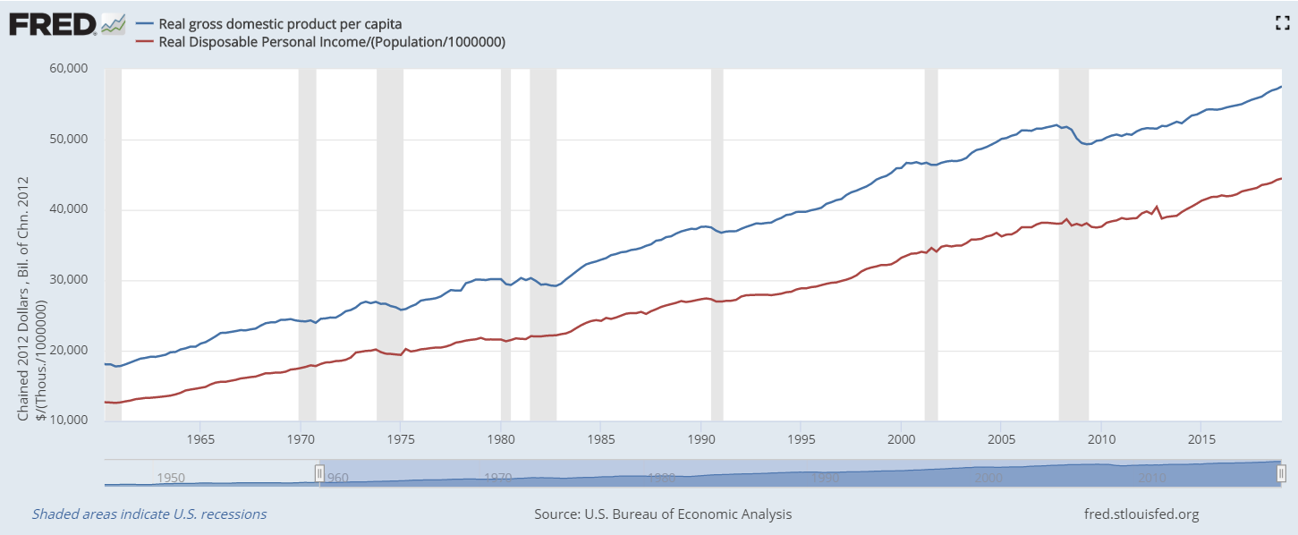
As you can see, labor is the majority input. In the following graph is the share of real GDP going to disposable income.  In the past two decades, labor has been getting a larger share.

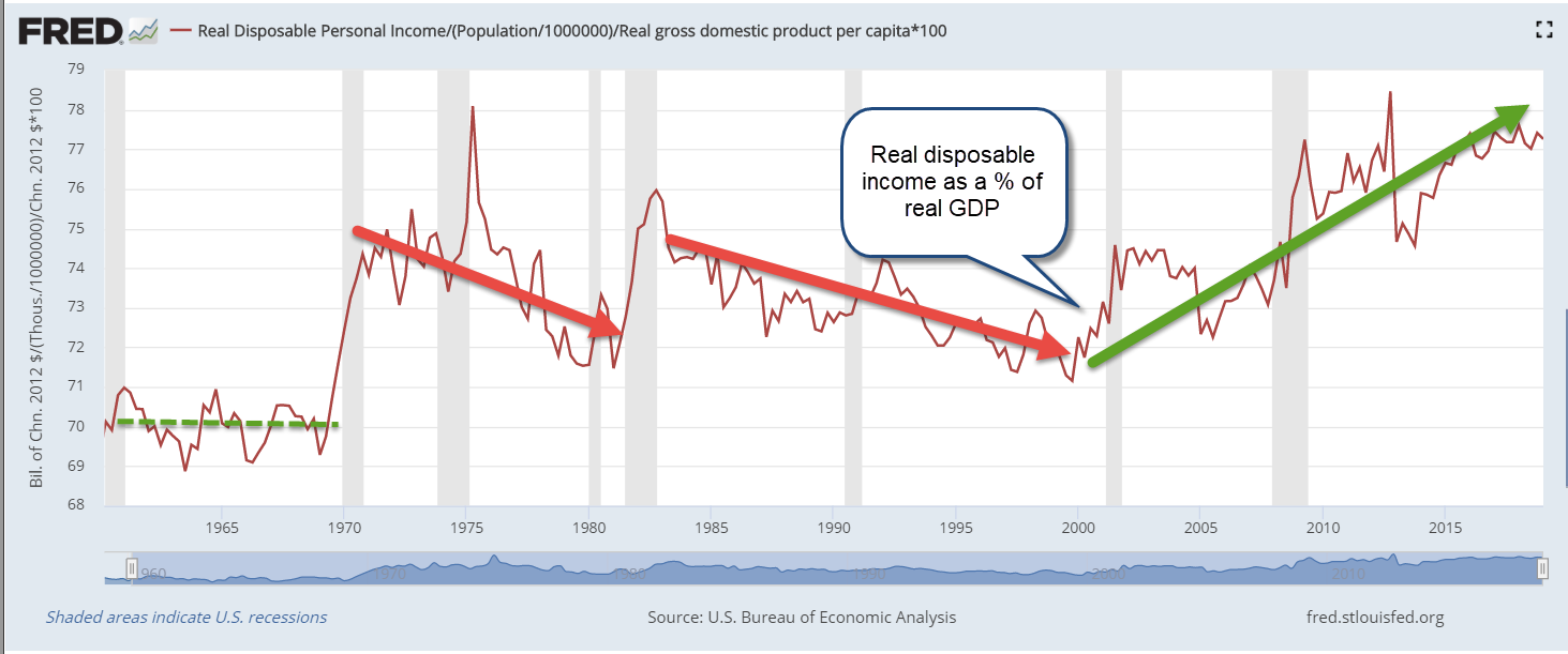
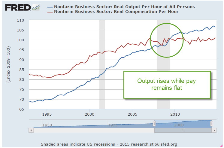
That might look good but it’s not. Since 2000, the economy has shifted toward service industries where labor does not produce as much GDP per hour. The chart below shows the efficiency of labor, or how much GDP is being produced by labor.

If labor were being underpaid, the amount of GDP produced per dollar of disposable income would be higher, not lower. On average, service jobs do not have as much leverage as manufacturing jobs.

A century ago, agricultural jobs were inefficient in comparison to manufacturing jobs. The share of labor to total output was high. In the past seventy years, the agricultural industry has transformed. Today’s farms resemble large outdoor manufacturing plants without walls and productivity continues to grow. In the past five years, steep price declines in the prices of many agricultural products have put extraordinary pressures on today’s smaller farmers. The increased productivity of larger farms has allowed them to maintain real net farm income at the same level as twenty years ago (Note #1). Here’s a graph from the USDA.

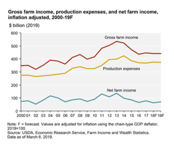
Although agriculture related industries contribute more than 5% of the nation’s GDP, farm output is only 1% of the nation’s total output. The productivity gains in agriculture have not been shared by the rest of the economy. Labor productivity has plunged from 2.8% annual growth in the years 2000-2007 to 1.3% in the past eleven years (Note #2).  Here’s an earlier report from the Bureau of Labor Statistics with a chart that illustrates the trends (Note #3). The report notes “Sluggish productivity growth has implications for worker compensation. As stated earlier, real hourly compensation growth depends upon gains in labor productivity.”

Productivity growth in this past decade is comparable to the two years of deep recession, high unemployment and sky-high interest rates in the early 1980s. The report notes “although both hours and output grew at below-average rates during this cycle [2008 through 2016], the fact that output grew notably slower than its historical average is what yields the historically low labor productivity growth.” Today we have low unemployment and very low interest rates – the exact opposite of that earlier period. Why do the two periods have similar productivity gains? It’s a head scratcher.

Simple answers? No, but hats off to Donald Trump who has called attention to the need for a greater shift to manufacturing in the U.S. economy. He and then Wisconsin governor Scott Walker negotiated with FoxConn Chairman Terry Gou to get a huge factory built in Mount Pleasant, Wisconsin to manufacture LCD displays, but progress has slowed. An article this week in the Wall St. Journal exposed the tensions that erupt among residents of an area which has made a major commitment to economic growth (Note #4).

If we don’t shift toward more manufacturing, American economic growth will slow to match that of the Eurozone. Along with that will come negative interest rates from the central bank and little or no interest on CDs and savings accounts. We already had a taste of that for several years after the recession. No thanks. Low interest rates are a hidden tax on savers. They lower the amount of interest the government pays at the expense of individuals who are saving for education or retirement. Interest income not received is a reduction in disposable income and has the same effect as a tax. Low interest rates encourage an unhealthy growth in corporate debt and drive up both stock and housing prices.

///////////////////

Note:

  1. USDA summary of agricultural industry
  2. BLS report on multi-factor productivity
  3. BLS report on declining labor productivity
  4. FoxConn LCD factory (March article – no paywall). Also, a recent article from WSJ (paywall) – Foxconn Tore Up a Small Town to Build a Big Factory—Then Retreated

Productivity And Labor Unions

February 5, 2017

About 10% of all workers, public and private, belong to a union. Today the percentage of private sector employees who are unionized is the same as in 1932, eighty years ago. (Wikipedia) The rise and fall of unon membership looks like the familiar bell curve, with the peak in the 1970s. The causes of the decline are debated but some attribute the erosion of union power as an important factor in wage stagnation.

The major factor is not declining union membership but declining productivity, and that persistent decline has economists and policymakers baffled.  Higher productivity should equal higher wage growth and, in the 30 year post-war period 1948-1977, multi-factor productivity (MFP) annual growth averaged 1.7%. MFP includes both labor and capital inputs. In the 40 year period from 1976-2015, MFP growth averaged about half that rate – .9%.

prodmfp1948-2015

In the debate over the causes of the decline, some contend that all the easy gains were made by 1980.  Productivity is now returning to a centuries long growth trend that is less than 1%. In an October 2016 Bloomberg article, Justin Fox picked apart BLS data to show that growth has been flat in some key manufacturing areas for the past three decades. The ten-fold surge in productivity growth in the tech sector is largely responsible for any growth during the past 30 years. OECD data indicates that other developed countries are experiencing a similar lack of growth (OECD Table) When no one can conclusively demonstrate what the causes are for the decline, policymakers face tough challenges and even tougher debate over the solutions.

//////////////////////////////

LoanGate

LoanGate may the next scandal. A few months ago, the Dept of Education (DoE) revealed that they had seriously undercounted student loan delinqencies because of a programming error. When the Wall St. Journal analyzed the revised data, they found that the majority of students at 25% of all colleges and trade schools in the U.S. had defaulted on their student loan or failed to make any repayment.  (WSJ article)

The Obama administration forced the closure of many private institutions whose students had low repayment rates. In 2015, Corinthian Colleges shuttered the last of its schools and filed for bankruptcy. The revised data show that many more institutions, both public and private, should be shut down.

This latest programming error at the DoE follows other embarrassing episodes during the two Obama terms. In October 2013, the rollout of Obamacare was riddled with programming errors that blocked many applicants from enrolling in a plan with healthcare.gov.

In 2010, the IRS delayed many applications for 501(c)3 tax status from mostly conservative political groups. Lois Lerner, the head of the agency, first claimed that these had been innocent clerical mistakes by an overworked staff, but a series of hearings uncovered the fact that employees at the IRS had acted on their own political feelings and deliberately targeted these groups. (Mother Jones)

In yet another incident, the Office of Personnel and Managment (OPM), the HR dept for thousands of Federal employees, revealed in 2016 a data breach involving 22,000,000 personnel records, including Social Security numbers.  Unchecked programming errors and data breaches erode the public’s faith in public institutions.  That these mistakes happened under a Democratic administration favoring ever bigger public institutions to solve ever bigger social problems is especially embarrassing.

When Obama first took office in 2009, the inflation adjusted total of student debt had quadrupled in the 15 year period (DoE paper – page 1) since 1993. By the time he left office eight years later, student debt had grown ten-fold to $1.3 trillion. The delinquency rate on that debt is 11% but the repayment rate is considered a better predictor of future delinquencies. The revised data reduced the combined repayment rate to a little more than 50% (Inside Higher Ed), far lower than the 75% plus repayment rates of a few decades ago.

The defaults are coming and there will be an inevitable call for a taxpayer bailout.  A popular element of Bernie Sanders’ Presidential platform was that a college education should be free. In the real world, nothing is free, so somebody pays.  Who should pay and how much will further aggravate tensions in an already divided electorate.

///////////////////////////////////

Five Year Rule

A few weeks ago I wrote about the 5-year rule, a backstop to any allocation rule. Any money needed in the next five years should be in stable assets like short to intermediate term bonds, CDs and cash. Why 5 years of income? Why not 2 years or 10 years? Answer: History.

Let’s look back at 80 years in 5 year slices, or what is called 5-year rolling periods. As an example, the years 2000 – 2004 would be a 5-year rolling period. 2001 – 2005 would be the next period, and so on.

Saving me the time and effort of running the data on stock market returns is a blogger at All Financial Matters who put together a table of this very data for the years 1926-2012. The table shows that the SP500 has held or increased its inflation adjusted value (very important that we look at the real value) almost 75% of the time. So the 5-year rule guards against a loss of value the other 25% of the time.

The 5-year rule can apply whenever there are anticipated income needs from our savings: retirement, college expenses, sickness or disability, and even a greater chance of losing our jobs. In a retirement span of 25 years, 6 of those years will fall into that 25% category. The 5-year rule minimum usually kicks in toward the end of retirement when a person’s reserves are lower and prudence is especially important.


Income, Housing and Durable Goods

In this week’s downturn, prices of the SP500 almost touched the 26 week, or half year, average of $203.90.  Since August 2012, when the 50 day average crossed above the 200 day average, these price dips have been good buying opportunities as the market has resumed its upwards climb after each downturn.

***********************

Manufacturing and Durable Goods

Preliminary readings of March’s Purchasing Managers’ Index (PMI) showed an uptick back into strong growth.  Survey respondents were concerned about weak export sales as the dollar’s strength makes American products more expensive overseas.  The full report will be released this coming Wednesday.

This past Wednesday’s report that Durable Goods had dropped 1.4% in February caused an already negative market to fall another 1.5% for the day and this marked the close of the week’s activity as well.  New orders for non-transportation durable goods have steadily declined since the fall.  Although the year-over-year comparisons are consistent with GDP growth, about 2.3%, the downward trend is concerning.

***********************
Housing

Existing home sales in February rose almost 5% in a year over year comparison, the best in a year and a half but still below the 5 million annual mark. The positive y-o-y gains during the past six months has prompted some optimism that sales may climb back above the 5 million mark in the spring and summer season.

New home sales in February surged back above a half million.  In a more healthy market, sales of new homes are 6% – 7% of existing homes.  In 2006, that ratio started climbing above the normal range, getting increasingly sicker until it reached almost 18% in May 2010.  February’s ratio was 9%. If the ratio were in the normal range, existing home sales would be over 8 million, far above the current 4.9 million units actually sold.

In a 2014 report the National Assn of Realtors noted that boomers tend to buy new or newer homes to avoid maintenance headaches while younger buyers buy older homes because they are less expensive (page 3).  38% of all home buyers are first timers but the percentage is double for those younger than 33 (Exhibit 1-9 in the report).  As the supply of existing homes is inadequate to meet the demand, prices climb and suppress the demand, forcing first timers to either buy a smaller new home or continue renting.

Sales of new homes and the fortunes of home builders are based on the churn of existing homes.  Since October, the stocks of home builders (XHB) have climbed 20% in anticipation of growing sales, but weak existing home sales may prove to be a choke point for growth.

The larger publicly traded homebuilders also build multi-family units.  Real investment in this sector has tripled from the lows of early 2010 but are still below pre-crisis levels.

The housing market in this country is still wounded.  63% of the population are white Europeans (Census Bureau) but are 86% of home buyers (Exhibit 1-6).  While few will admit to racial prejudice in the current housing market, the numbers are the footprints of this nation’s long history of racial discrimination and socio-economic disparity.  Mortgage companies that made – let’s call them imprudent – credit decisions that helped precipitate the housing crisis are especially cautious, making it more difficult for younger buyers to purchase their first home, despite the historically low mortgage rates.  This market will not heal until mortgage companies relax their lending criteria just a bit and that won’t happen while rates are so low.

**************************
Income

The Bee Gees might have sung “Words are all I have to take your heart away” because they were singing about love, not economics and finance.  Graphs often tell the story much better than words.  A milestone was passed a few years back.  For the first time since World War 2, the growth in income crossed below the growth in output.

This past week, the Bureau of Labor Statistics released a revision to their initial estimate of multi-factorial productivity in 2013.  There is a lot of data to gather for this series.  An often quoted productivity growth rate calculates the GDP of the nation divided by an estimate of the number of hours worked, a statistic that is accessible through payroll reports submitted monthly and quarterly.  The contribution of capital to GDP is much more difficult to assess and is largely disregarded by those like Robert Reich, former Secretary of Labor under President Clinton, who have a political axe to grind.  Truth is on a path too meandering for politics.

Total output in the years 2007 – 2013 was just plain bad, growing at an annual rate of only 1%, a third of the 2.9% growth rate from the longer period 1987 – 2013.  In the BLS assessment, the growth rates of both labor and capital inputs were poor by historical norms but capital input accounted for all of the meager gains in non-farm business productivity.  People’s work is simply not contributing as much to growth as before.  That reality means that income growth will be meager, which will prompt louder political rhetoric to make some kind of change, any kind of change, because voters like to believe that politicians have magic wands.