The Madness of Methodology

April 28th, 2013

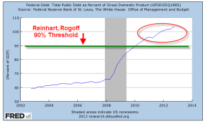
A fight between economists is not as exciting as a dinosaur smackdown (Jurassic Park), but the controversy can be as damaging.  Politicians and pundits love to trot out those economic studies and theories which justify their actions or political point of view.  In 2009, two economists Carmen Reinhart and Kenneth Rogoff (now affectionately known as RR), published a study which showed that a country’s GDP growth becomes slightly negative when its debt grows above 90% of its GDP.  The study was cited by many politicians and pundits in Europe and the US, including VP candidate Paul Ryan, as they proposed various forms of austerity to curb the explosive growth of national debt.

Here’s what the debt to GDP ratio looked like 1940 – 1960

In the years 1947 – 1959, we had an annualized growth rate of 3.6% but a strong component of this growth was our strategic advantage in exports, being the manufacturing capital of the world after much of the production capacity of the developed world was destroyed in WW2.

Here’s what it looks like now; the same spike of debt.

But we have lost the advantage of being the leading manufacturer.

Given the assignment of replicating an existing economic study, Thomas Herndon, a PhD candidate at UMass, discovered some glaring spreadsheet errors in the original data set compiled by RR.  You can read an Alternet article summarizing the details here.

Some quick background.  There are two categories of economic policies.  Fiscal policy encompasses taxing and spending measures by a government.  Monetary policy is conducted by a country’s central bank and are targeted at the supply of money and interest rates.  Economists argue over which policy is more effective in a given circumstance.  Each of us goes about our daily lives under the influence of both fiscal and monetary policy. 

During the 1930s depression, the economist John Maynard Keynes proposed that governments borrow and spend money during recessions to make up for the lack of aggregate demand in the economy.  After the economy recovered, governments would then raise taxes to pay back the borrowed money.  Another leading economist, James Buchanan, predicted that nations who followed Keynes’ ideas would have permanent deficits.  While Keynes’ economic model was elegant, Buchanan argued that there was no incentive for a politician to raise taxes.

In 1963, with the publication of A Monetary History of the U.S., economists Milton Friedman and Anna Schwartz argued that the Depression had been largely a result of failed monetary policy by central banks.  During the 1970s, when government fiscal policies of increasing intervention in the economy failed to ingnite growth or curb inflation, Keynes’ policies fell into disfavor. 

The age old debate about the effectiveness of fiscal and monetary policy never dies. The recession that began in 2008 revived Keynes’ ideas.  In the late 1990s and early 2000s, economist Paul Krugman and Federal Reserve chairman Ben Bernanke were proponents of monetary solutions for Japan’s moribund economy.  As the world economy imploded in 2008, both men changed course and became advocates for fiscal policy as the most effective solution for the country’s economic woes.

In a recently published paper UMass professors Michael Ash and Robert Pollin (Herndon’s advisors), explained their methodology and took RR to task for their lack of follow up on incomplete data analysis after several years.  What they had missed was a follow up paper by RR in February 2011 and another published in the summer of 2012.  In these papers, RR modified their initial findings, saying that GDP growth slowed but did not necessarily turn negative.

In a WSJ blog post , RR answered the critique from the UMass Professors.  They admitted their spreadsheet error but reaffirmed their other assumptions in the study and their amended conclusions.

Paul Krugman weighed in (or waded in?), voicing his disappointment with RR’s methodology and their conclusion.  Krugman does make a point oft repeated in the social studies: correlation is not causation.  Does high debt cause slow GDP growth?  Or, does slow GDP growth cause high debt?  Or can we say that there is some indication that they accompany each other?

At Econbrowser, U. Cal professor James Hamilton, reviewed RR’s methodology and Ash and Pollin’s critique. (Link)  To which, Professors Ash and Pollin responded with some good points.

Ash and Pollin have made the original data available.  Some have accused RR of purposefully leaving five countries out of their data, saying that these five countries would have weakened or invalidated their findings.  The Excel file shows that this was a simple – but dumb – mistake, not some nefarious plan by RR.  The countries left out are on the last five worksheets which are arranged in alphabetical order.  What surprises many is that two prominent economists could publish a paper based on work that had so little verification before publication. 

What I question is RR’s decision to include many of the smaller countries at all in their analysis.  Finland and Ireland each have less than 2% of the GDP of the U.S. 

What I do hope is that this controversy will spur more analysis of the relationship between a nation’s debt load and its economic growth.  What I am afraid of is that this will discourage researchers from sharing their working data.  Reinhart and Rogoff are to be highly commended for doing so.

GDP, Profits and Labor

Feb. 2nd, 2013

A lot to cover this week – the monthly labor report and the Dow Industrial Average breaks the psychological mark of 14,000.  Let’s cover the stock market rise because that will give us some context for the labor report.

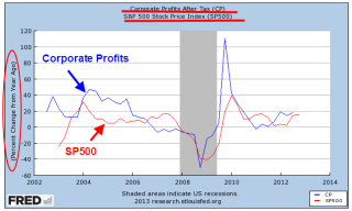
The stock market rises and falls on the prospect for the rise and fall in corporate profits.  For the past year, profits have been healthy, increasing year over year by 15-20%.

The stock market is a compilation of attempts to anticipate these profit changes by six months or so. Sometimes it guesses wrong, sometimes it guesses right but the market loosely follows the trend in profits.

As a percent of GDP, corporate profits have reached a record high and this growing share of the economy is largely responsible for the doubling of the SP500 in the past three years.

There can be too much of  a good thing and this may be it.  An economy becomes unstable as one segment of the economy accumulates a greater share of the pie.

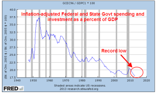
Facts are the nemesis of partisan hacks who simply disregard any information that does not fit with their model of how the universe works.  Data on government spending and investment contradict those who complain that government has too much of a share of the economy; it is now at historic lows.

This includes government at all levels: federal, state and local.  Reductions in government spending continue to act as a drag on both GDP and employment growth. What gives some people the sense that government spending is a larger percentage of the economy are transfer payments, like Social Security.  Neither the calculation of GDP or government spending includes these transfer payments, so the percent of government spending in relation to GDP as shown in the chart above is a truer picture of government’s role in the economy. 

Speaking of GDP – this past week came the first estimate of GDP growth for the fourth quarter of 2012.  The headline number was negative growth of 1/10th of a percent on an annualized basis.

Two quarters of negative growth usually mark the beginning of a recession.  Concern over this negative growth led to small losses in the stock market at mid-week as investors grew concerned about the January labor report, which was released Friday.  The negative growth was largely due to a severe reduction in defense spending and exports.  As a whole, the private economy grew at an annualized rate of 3.6%, a strength that helped moderate any market declines in mid week.

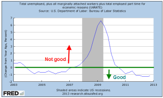
When the Bureau of Labor Statistics released their monthly labor report this past Friday, the headline job increase of 157,000+ and an unemployment rate stuck at 7.9% did not calm investors’ fears.  The year over year percent change in unemployment is still in positive territory.

The numbers of long term unemployed as a percent of total unemployment ticked down but remains stubbornly high at about 38% (seasonally adjusted)

What prompted Friday’s relief rally in the market were the revisions in the previous months’ employment gains.  As more data comes in, the BLS revises previous months’ estimates.  This month also included end of the year population control adjustments.

November’s gains were revised from +161,000 to +247,000; December’s gains were raised from +155,000 to +196,000.  For all of 2012, the revisions added up to additional job gains of 336,000, raising average monthly job gains for 2012 to 181,000 – near the benchmark of 200,000 needed to make a dent in the unemployment rate.  Previous decreases in the unemployment rate have been largely the result of too many people giving up looking for work and simply not being counted as unemployed.

Overall, the labor report put the kibosh on any fears of recession and the stock market responded with a rally of just over 1%.  Construction jobs continued their recent gains but employment levels are one million jobs fewer than the post-recession lows of 2003 and two million jobs less than the 2006 peak of the housing bubble.

The core work force aged 25-54 continues to struggle along.

The older work force has garnered much of the gains in the past year but this month was flat.

The larger group of workers counted as unemployed or underemployed, what is called the U-6 Rate, remained unchanged as did the year over year percent change. 

As the stock market continues to rise, retail investors have reversed course and have started to put more money into the stock market.  Sluggish but steady GDP and employment growth has prompted the Federal Reserve to continue its program of buying bonds every month, which tends to push up stock market values.  The Fed can continue this program as long as the sluggish pace keeps inflation in check and below the Fed’s target rate of 2.5%. 

In the short run, it is a good idea to follow the maxim of “Don’t Fight the Fed.”  What is of some concern is the long term picture.  Below is a 30 year chart of the SP500 index, marked in 10 year periods with two trend lines based on the first decade, one trend line (with the arrow) a bit more positive than the other. 

The market has changed in the past two decades.  The bottoms in 2002, 2003, 2010, 2011 were simply a return to trend, a return to sanity.  The downturn of late 2008 – early 2009 was the only downturn that broke below trend; truly, an overcorrection. Among the changes of the past two decades is a Federal Reserve that, some say, has helped drive these erratic asset bubbles by making aggessive interest rate moves, then keeping interest rates at low levels for a prolonged period of time.  Whether and how much the Fed’s interest rate policies contribute to stock market valuations is a matter of much vigorous discussion.  Whatever the causes are, it is important to recognize that over two decades the market has shifted into a jagged, cyclic investment.  The long term investor who has a ten year time frame before they might need some of the money invested in the stock market can be reasonably certain that they will be able to get most of their money back if not make a healthy profit.  For those with a shorter time horizon like five years, they will need to monitor the financial and economic markets a bit more closely or hire someone to do it for them.  This is especially true when one is buying at current market levels which are above trend.

GDP and Recession

So you’re sitting at a picnic table in the park, having a barbecue with friends and family and one of your kids starts complaining about how life is so unfair because of something or other and you find your mind drifting off to the state of the economy.  You feel like telling your kid that, as they grow older, they are going to find that life is full of unfair and to just get over it.  But you don’t tell your kid that because they are not strong enough for it yet, which reminds you of Jack Nicholson’s line in the movie A Few Good Men: “You can’t handle the truth!”  But you don’t tell that to your kid because it would scare them so you act sympathetic and give your kid a little hug and pretty soon everything is OK again except that about eight feet away from the table Uncle Bob is having an argument with your friend about the money the government is spending.

Uncle Bob is saying that Obama and the Democrats are bringing down this country and your friend counters that it is Obama who trying to resurrect the country after Bush’s eight years as President.  You begin to turn your shoulders to them as though to insert yourself into the debate but notice that your wife is looking at you kinda funny from across the picnic table and, while you are not that good at mind reading, there is something in her look that raises a flag of caution in your mind.  Your father in law is busy at the barbecue and calls out that the burgers will be ready in five minutes – which gives you just enough time to whip out your iPad and check the Federal Reserve data site to answer a nagging question:  what is GDP per person in this country?

Gross Domestic Product accounts for most of the private and government economic activity in a country.  GDP doesn’t take into account the money that a government borrows to fund its spending;  GDP only includes the spending.  GDP doesn’t care what the money was spent for, whether it was to build a bridge in Iowa or destroy a bridge in Afghanistan.  Regardless of these and other faults,  GDP serves as a report card on a country’s economy.

Real GDP is an inflation adjusted GDP, a way of comparing apples to apples over the years.  Real GDP per capita is the inflation adjusted economic output per person.

You type in “Real GDP” into the search box  and the Federal Reserve database, or FRED to its many users, obliges you with a list of GDP reports and you select the first one. The full graph comes up showing the years 1947 to 2012.  You touch the Edit Graph button, then change the beginning date to 1960.

Both Uncle Bob and your buddy have had a few beers, a beverage which adds certainty to a man’s opinion.  You wonder how many of these political-economic debates have occurred this week at the dinner table, at the office, while taking a break on a construction site.

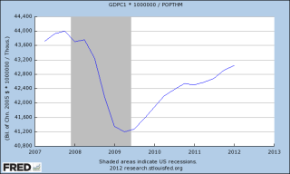
Your iPad screen shows the rise in real GDP with the “hook” starting in late 2007.  It is that hook that has got a lot of people arguing.  Its the hook that has pulled home values down and given a hard yank on the retirement dreams of  many people.  That hook tugged away the after school program your kid was in as the school district tightened its belt.  That hook took your wife’s job away; it almost took yours.

Now your buddy is talking loudly and pointedly about higher education cuts, but is barely able to finish his sentence as Uncle Bob interrupts him with the tale of the state university vice-president who is getting $300K a year in pension benefits.  Bob is sick of paying higher taxes for the fat cat retirements of the elite government employees.

Although the Bureau of Economic Analysis called an end to the recession in June of 2009, every adult with half a brain knows that the recesson didn’t end then. The billionaire investor Warren Buffett uses a rule of thumb that a recession ends when real GDP gets above the high point before the recession began.  You touch the “5 year” range button on the screen and see that real GDP has in fact surpassed that high point in 2007 so Buffett probably called and end to the recession in the fall of 2011.


FRED conveniently colors in the recessions, highlighting the periods in gray, but they are the “official” periods of recession, when GDP rises or falls for two consecutive quarters.  GDP could fall from $100, for example, to $60, signalling a recession, then increase to $65 over six months and the BEA would say it was the end of the recession, even though any sane person would say “Hey, we’re still down a third from the $100 high point.”

Has the GDP per person surpassed its 2007 high?  Your mother-in-law leans over and asks whether you want lettuce and tomato, glances down at the iPad screen with just a hint of disapproval in the set of her mouth and tells you that everyone will be eating soon.  OK, just a minute, you tell her.

Touching the screen, you click the “Add Data Series”, then touch line 1.  In the box you type “POPTHM”, the population census figures.  The other night, you couldn’t remember Bruce Willis’ name from the Die Hard movies but you can remember the label for the population series.  You’re not old yet but this is probably what happens to old people’s brains.  To get the GDP, which is in billions, per capita, which is in thousands, you need to multiply the GDP dollars by a million before dividing so you type into the formula box: “a * 1000000 / b” and touch the “Redraw Graph” button below it.

FRED redraws the graph, showing that the per capita GDP has still not risen above the 2007 high point.


For four and half years we have been in recession, you think.  No wonder we are arguing.

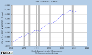
Was it as bad as the recession in the early eighties, you wonder.  That was a double dip recession.  You touch the starting date box and click on 1960 and a new expanded graph appears on the screen. “Hey, hon, why don’t you help me with the ice?” your wife asks.  “Ok, just a sec,” you reply, not looking up from the screen.

You see that this recession on a per capita basis is about the same as the early eighties, lasting about four and a half years, from late 1978 to mid 1983, with an upward hiccup during that period.  The period was the same but the decline in the late 70s and early 80s was much shallower than this current recession. 

You want to show both your friend and Uncle Bob why they are arguing, that the recession really hasn’t ended, the comparison of this recession and the 1980s but your wife needs help with the ice so you close the iPad cover.  Maybe you can show them the graph after the meal.  “Burgers are up!” your father-in-law shouts and the whole group sits down to chow down. 

After the meal, your friend hauls out an old croquet set. There are a few hoops missing and one mallet has a head but no handle, but the kids are delighted.  At some point in the game, Uncle Bob sends your friend’s ball far afield with a taunt “Out in left field where the liberals belong!” but your friend doesn’t take the bait.  On second thought, you muse, showing these guys the graphs would only reignite the debate.

“Daddy, it’s your turn.  You can use my mallet,” your kid says and you reach for the mallet, thinking  We try to teach our kids to be considerate and cooperative on the playground and in school.  So what happens to that sense of cooperation when we grow up?

Obama’s GDP Problem

In these home stretch months before the election, President Obama and Republican nominee Mitt Romney will be repeatedly challenging each other’s economic performance; Obama as President and Romney as Governor of Massachusetts.  Already the initial attack ads of both campaigns are running and each has plenty of factual ammo they can aim at the other.  Contrary to all common sense, we continue to measure Presidents by the health of the economy.  Although Congress is largely responsible for the laws that govern the economic dynamo of a country, we look to the President to set priorities for Congress – or at least that’s what we tell ourselves.  In truth, we are rather simple minded and prefer to hold one man responsible rather than a group of 535 Congress people and Senators. 

For some background, let’s take a look at a chart showing the real GDP, that is GDP in constant 2010 dollars, per capita over the past five decades.

Then zoom in on the last ten years, showing the severe decline of per capita GDP during this recent recession.

Now let’s look at the total per capita GDP growth by President.  If real GDP per capita was $100 when a President took office and $120 when he left office, then total real GDP growth was 20% during that President’s watch.  We’re not going to look at the annual percentage of growth, only the total.  For the most recent GDP data I have used BEA estimates of $15,454 trillion as of the first quarter of 2012. I have used Census Bureau estimates of a total population of 313 million and a BLS inflation factor of 2.186 since 2010.

Almost by instinct, the voters do not re-elect Presidents who are at the helm of a low growth country.  Below is a chart of the first term total real GDP growth of Presidents who were re-elected.  I have not included Johnson because he only served for a year before he was re-elected.

As you can see, GW Bush was the only President re-elected with a total growth gain less than 10% and Bush won re-election by winning Ohio by two percentage points or 118,775 votes.  Had 60,000 voters cast their ballot for Kerry, GW Bush would have lost Ohio’s 20 electoral votes and the election.  As the first Presidential election after 9/11, the election focused more on national defense and foreign policy, not the economy.  A barrage of attack ads, the Swift Boat campaign, against Kerry in the last weeks leading up to the election proved to be a decisive factor in Bush’s re-election.  Had the election concentrated more on the economy, Bush probably would have lost the election.

I have listened to several conservative pundits who criticize Obama for continuing to run against Bush’s economic policies, contending that it has been 3-1/2 years since Obama took office.  Many conservatives are devotional acolytes of the Ronald Reagan legacy and their devotion often clouds their memory.  Obama is using the same strategy that Reagan did in 1984, who ran against Carter’s former Vice President, Walter Mondale.  I will paraphrase a common refrain of Reagan during his re-election bid: “Do you want someone (Mondale) who helped get us in this mess in the first place?” Reagan asked.  The voters answered a resounding “No” and sent Mondale down to a crushing defeat.  Reagan employed this tactic of running against a former President despite the relatively strong growth during his first term. 

Although Obama’s total GDP growth is better than GW Bush’s total, it is less than former President Carter, a guy who lost his job over relatively weak growth and Obama’s 1st term growth numbers are less than Bush’s first term growth. A strong 1st quarter of economic growth in 2012 has helped pull up the President’s economic growth numbers but the first reading of 2nd quarter GDP growth that comes in July may further weaken his chances just before the election.  By the time 3rd quarter GDP numbers come out in October, many voters will have already made up their minds.

For his part, Romney’s tenure as governor of Massachusetts was hardly exemplary.  We will have two contenders for the Presidency running on an economic platform and neither one of them has a strong record of economic growth while in office.  Both campaigns will have plenty of arrows in their quivers and each candidate presents an inviting target.  Enjoy the show!

Debt Comparison

As this past quarter began in July, Greece’s debt was a concern but the countries of the EU were in negotiations to work it out.  QE2, the Federal Reserve’s program of bond buying, had just ended, prompting some to worry about a negative effect on the economy as that stimulus.   Early second quarter earnings reports in mid July were strong and the balance sheets of major companies showed that they had accumulated ample reserves of cash to weather any small downturns. Manufacturing was slumping a bit but that was attributed to supply chain disruptions from the March Japanese tsunami and was expected to grow again in the third quarter.  The moribund housing sector and stubbornly high unemployment remained a concern but the stock market is a pricing of future company earnings.  The companies in the S&P500 which have any foreign earnings receive the majority of their earnings from countries other than the U.S.  This global sales and revenue base makes these large U.S. companies less vulnerable to economic weakness in any one country.

Japan’s recovery in GDP in the second quarter surprised many, testifying to the resilience and industry of the Japanese people and Japanese industry.  China, Indonesia, India and Brazil were showing strong growth, perhaps a bit too much growth, as inflation in those countries and regions was prompting central banks to take steps to cool that growth.  Growth in the EU countries was a concern but German manufacturing was holding steady.

Toward the end of July, the EU reached an agreement to provide financing to Greece and, in the U.S., President Obama and House Speaker Boehner supposedly reached an agreement – dubbed the “grand bargain – for debt reduction.  On July 22nd, the S&P500 closed near 1350.  At the end of September, the S&P500 stood at 1130, a drop of 17%.  What happened?

The weekend after the “grand bargain” came news that there was no bargain.  During August, the American people stared in befuddlement at a dark comedy in which lawmakers and the President brought the country to the brink of default, prompting one rating agency to downgrade U.S. government debt. 

Computing the Gross Domestic Product (GDP) of an entire nation is a complex affair, one that requires an early estimate and two revisions. In the late days of July, the Bureau of Economic Analysis (BEA) revised the GDP growth for the 1st quarter of 2011 (ending in March) from a weak 1.9%  to an almost recessionary .4%.  This was a large revision and shook the markets, swiftly dropping the S&P500 index to about 1100. 

Germany reported strong manufacturing data for July but China showed a stalled growth in their manufacturing, adding to worries about a global slowdown.  Since early August, the market has behaved like a small boat in the Mid Atlantic, rising and falling dramatically with both news and worries about Greece’s debt as well as the debt of Italy, Spain, Ireland and Portugal.  Investors have fled from the stocks of banks holding the debt of those countries as well as larger banks which might have indirect exposure to that debt.  An index of large banks has fallen 28% since April of this year.  Many developed countries are wallowing in debt.  A slowdown in growth leads to less tax revenue to pay down that debt.  Worries of a global recession or a severe slowing of growth provoke fear of bank defaults, government defaults, and growing pressure on small and medium sized businesses, who are least able to withstand downturns in an economy.

Fractious meetings among EU member countries, among the various branches of the U.S. government leads many to regard politicians on both sides of Atlantic as dysfunctional, unable to resolve their ideological differences to make any functional policy decisions.  Investors worry about the viability and future of the euro currency, fleeing the Euro and parking their money in U.S. Treasuries, causing the price of Treasuries to rise and the yield (interest) on those bonds to fall to historically low levels.

In September, an HSBC index of small and medium Chinese manufacturers reported a slight contraction.  German manufacturing declined from strong numbers in July to a neutral stall speed in September, confirming fears of a global slowdown. 

In the U.S. and Eurozone, governments at all levels have instituted austerity measures to cope with declining tax revenues.  Government employee layoffs increase the demand for social support programs, prompt civilians to curb their spending, resulting in less tax revenues for government, prompting more government cuts, ad nauseum.  Cautious companies hoard what cash they have, reduce their investments in anticipation of further slowdowns in consumer demand.

Weighing on the economies of the U.S, Japan and Europe are a decades long accumulation of debt.  Below is a chart of OECD data on the total debt of developed countries.  Debt in the U.S. doesn’t look bad compared to some of these other countries. (Click to enlarge in separate tab)

For the past thirty years, all of us in the U.S. have been running up debt.  People, companies and governments at the Federal, State and local levels have borrowed…and borrowed…and borrowed some more. 

The severely slumping U.S. housing market is a strong headwind to any GDP growth.  Lower valuations lead to less property taxes for local governments and schools, reduced government services, houses that are difficult for homeowners to sell without bringing cash to the sale. A recent report by the Commerce Dept. showed that housing has contributed an average of 4.7% to GDP for the past half century.  Last year, housing contributed only 2.2% to GDP.  If the health of the housing sector was just average, GDP growth in this country would be 2.5% higher.   Some in the industry anticipate that it will be another five years for housing to recover from the excesses of the past decade.

Recession Procession

Recently, the National Bureau of Economic Research (NBER) made their official pronouncement that the recession that began in Dec. 2007 ended in June 2009. In July 2009, the Federal Reserve had issued its unofficial estimation that the recession had just ended. This latest announcement by the NBER is a statistical confirmation of what the Federal Reserve had announced over a year ago. To many individuals and businesses, however, the recession is not over. In a CNBC interview, the renowned investor and billionaire Warren Buffett stated his more common sense definition that the recession is not over until production and income get back to the levels they were before the recession started. Most would agree.

There is no clear definition of the beginning and end of a recession but the NBER’s Business Cycle Dating Committee states that a recession is “a significant decline in economic activity spreads across the economy and can last from a few months to more than a year.” The rule of thumb is two consecutive quarters of negative GDP growth. But neither the NBER definition or the rule of thumb adequately captures the effect – how it feels – of a downturn in the economy. That is because the rule of thumb is based on quarter to quarter growth or decline in GDP. If GDP were a $1 and, over a year, fell to 80¢, then rose to 85¢ in the following quarter, the economy would still be terrible but the growth in GDP would be an annualized 25%. For this reason, Buffett’s rule of thumb gives a more accurate picture.

Below is a NBER chart of real, or inflation-adjusted GDP, with Dec 2007 being the benchmark of a 100. As you can see, our economy is still below the level of December 2007. (Click to view larger image in a new tab)

The severe downturn in manufacturing and retail sales tells a more complete picture, not only of the national economy, but the state and local economies which depend heavily on sales taxes for their revenue. Total unemployment is about 16% of the workforce and, until that situation improves, there will be only sluggish growth in sales, which in turn will keep on damper on GDP growth.

The Drifters

Matt brought up some good questions and comments yesterday.  I’ll look at one aspect that he brought up – the stagnation of wages for the past 35 years.

Over the past 3 to 4 decades, the U.S. economy has been transitioning to an almost entirely service based economy.  In 1953, manufacturing was 28% of the economy, a post WW2 high.  By 1995, it was only 16% of the economy, and by 2007 it had sunk to 12%.  How has this decades long shift affected the nation’s GDP?

Below is a graph of U.S. GDP 10 year averages since WW2 and the averages for the periods 1946 – 1972 and 1973 to 2009.  (Click to enlarge)

Source:  Bureau of Economic Analysis

As you can see, average GDP growth has declined in the last 35 years by 12% from the 25 year period after WW2. I have heard Ben Bernanke, chairman of the Federal Reserve, say that they like to see an overall 3.0% average growth of GDP for a healthy economy – not too hot, not too cold. For the past 35 years, we have been just shy of that.

In this next chart, I combined data from the Bureau of Economic Analysis and the Census Bureau to show real GDP per capita growth  in 2009 dollars. 

In this next chart, I’ve drawn trend lines to show the various “speeds” of real GDP per capita growth over the past 60 years.  As you can see, the growth trend of the last 30 years or so has been below the growth trend of the 1960s.  The data also reveals that the 60s was an anomaly – a decade of robust growth that was partially fueled by military spending.  Yet it is this decade that some use as a baseline of comparison – a golden age of increased productivity and increased wages.

Although the growth of the past 3 decades might not be what it was during the 60s, it still averages 2.8%.  Have workers seen any of those gains in growth?  According to the BLS, the 1987 average hourly cost, including benefits, for workers in private business was $13.25, or $26.37 in 2009 dollars.  In March 2010, the BLS reports the average hourly cost at $29.71.  Over the past 24 years, companies have seen their real employee costs rise by only 13%, or about 1/2 percent a year.

During that same period, benefits have risen from 27% of total employee cost to 30%. Despite a 50% increase in inflation adjusted costs for health care in the past decade, businesses have managed to hold their labor costs down.  How have businesses managed this?  By reducing average wages.  In 1973, average hourly earnings for employees in private business was $4.14 ($20.00 in 2009 dollars).  In 2009, average hourly earnings were $18.62.   In real inflation adjusted dollars, workers have gained a tiny bit in benefits and lost about 5% in wages over the past 35 years.  Workers have simply not enjoyed either the gains in GDP growth or the gains in productivity over the past 3 decades or more.

But the pain felt by hourly and salaried workers is aggravated by the decline in work hours.  The BLS reports  that average weekly hours was 36.9 in 1973.  In 2009 weekly hours averaged only 33.1.  The reduced hours has affected the average worker’s weekly total.  In 1973 it was $152.77, or $738 in 2009 dollars.  In 2009, it was $617, a real drop of 16%.

How have business owners been able to keep a lid on worker wages for these past 35 years?  Supply and demand.  As I noted above, GDP growth has lessened over the past three decades, reducing demand.  During that period, the supply of labor has increased. In 1973, the BLS reports that there were 64 million in the civilian workforce, 40 million men and 24 million women.  The civilian workforce was 30% of the population of 212 million.  In 2008,  the total civilian workforce had almost doubled to 125 million, 67 million men and 58 million women.  This workforce was 41% of the total population of 304 million.  Look at the ratio of men to women in the workforce.  In 1973, there were almost two men for each woman.  By 2008, the ratio approached a one-to-one ratio. As more women entered the workforce, they put downward pressure on wages, which induced more women to enter the workforce to make up for lost household income.  This cycle will continue for the next two decades unless this country decides to implement policies that will return some of the lost manufacturing capacity to this country.