Pocketbook Ratios

January 21, 2024

by Stephen Stofka

Thanks to an alert reader I corrected an error in the example given in the notes at the end.

This week’s letter is about the cost of necessities, particularly shelter, in terms of personal income. Biden’s term has been one of historic job growth and low unemployment. Inflation-adjusted income per capita has risen a total of 6.1% since December 2019, far more than the four-year gain of 2.9% during the years of the financial crisis. Yet there is a persistent gloom on both mainstream and social media and Biden’s approval rating of 41% is the same as Trump’s average during his four-year term. Even though there are fewer economic facts to support this dour sentiment, a number of voters are focusing on the negatives rather than the positives.

I will look at three key ratios of spending to income – shelter, food and transportation – to see if they give any clues to an incumbent President’s re-election success (a link to these series and an example is in the notes). Despite an unpopular war in Iraq, George Bush won re-election in 2004 when those ratios were either falling, a good sign, or stable. Obama won re-election in 2012 when the shelter ratio was at a historic low. However, the food and transportation ratios were uncomfortably near historic highs. These ratios cannot be used as stand-alone predictors of an election but perhaps they can give us a glimpse into voter sentiments as we count down toward the election in November.

A mid-year 2023 Gallup poll found that almost half of Democrats were becoming more hopeful about their personal finances. Republicans and self-identified Independents expressed little confidence at that time. As inflation eased in the second half of 2023, December’s monthly survey of consumer sentiment conducted by the U. of Michigan indicated an improving sentiment among Republicans. The surprise is that there was little change in the expectations of Independents, who now comprise 41% of voters, according to Gallup. There is a stark 30 point difference in consumer sentiment between Democrats and the other two groups. A recent paper presents  evidence that the economic expectations of voters shift according to their political affiliations. A Republican might have low expectations when a Democrat is in office, then quickly do an about face as soon as a Republican President comes into office.

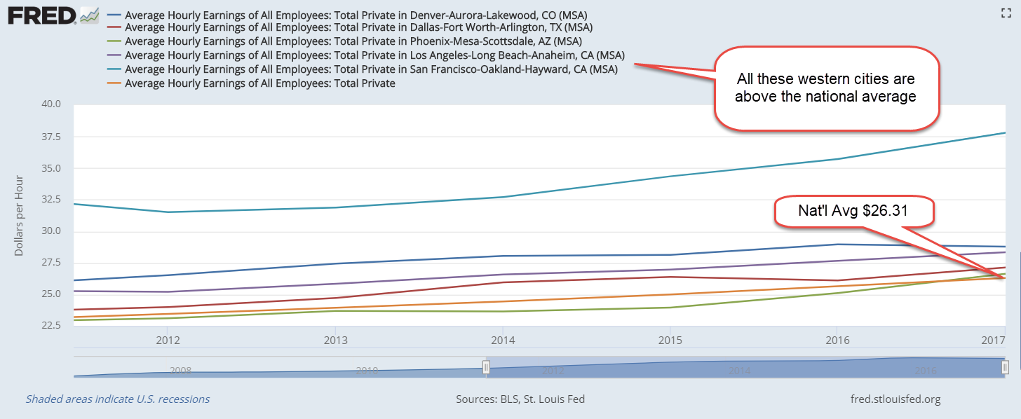
Shelter is the largest expense in a household budget. Prudential money management uses personal income as a yardstick. According to the National Foundation for Credit Counseling, the cost of shelter should be no more than 30% of your gross income. Shelter costs include utilities, property taxes or fees like parking or HOA charges. Let’s look at an example in the Denver metro area where the median monthly rate for a 2BR apartment is $1900. Using the 30% guideline, a household would need to gross $76,000 a year. In 2022 the median household income in Denver was $84,000, above the national average of $75,000. At least in Denver, median incomes are outpacing the rising cost of shelter. What about the rest of the country?

The Bureau of Labor Statistics (BLS) calculates an Employment Cost Index that includes wages, taxes, pension plan contributions and health care insurance associated with employment. I will use that as a yardstick of income. The BLS also builds an index of shelter costs. Comparing the change in the ratio of shelter costs to income can help us understand why households might feel pinched despite a softening of general inflation in 2023. In the graph below, a rise of .02 or 2% might mean a “pinch” of $40 a month to a median household, as I show in the notes.

Biden and Trump began their terms with similar ratios, although Biden’s was slightly higher. Until the pandemic in early 2020, housing costs outpaced income growth. Throughout Biden’s first year, the ratio stalled. Some states froze rent increases and most states did not lift their eviction bans until the end of July 2021. In 2022, rent, mortgage payments and utility costs increased at a far faster pace than incomes. Look at the jump in the graph below.

An economy is broader than any presidential administration yet voters hold a president accountable for changes in key economic areas of their lives. Food is the third highest category of spending and those costs rose sharply in relation to income.

Transportation costs represent the second highest category of spending. These costs have risen far less than income but what people notice are changes in price, particularly if those changes happen over a short period of time. In the first months of the pandemic during the Trump administration, refineries around the world shut down or reduced production. A surge in demand in 2021 caused gas prices to rise. Despite the rise, transportation costs are still less of a burden than they were during the Bush or Obama presidencies.

Neither Biden nor Trump were responsible for increased fuel costs but it happened on Biden’s “watch” and voters tend to hold their leaders responsible for the price of housing, gas and food. In the quest for votes, a presidential candidate will often imply that they can control the price of a global commodity like oil. The opening of national monument land in Utah to oil drilling has a negligible effect on the price of oil but a president can claim to be doing something. Our political system has survived because it encourages political posturing but requires compromise and cooperation to get anything done. This limits the damage that can be done by 535 overconfident politicians in Congress.

Voters have such a low trust of Congress that they naturally pin their hopes and fears on a president. Some are single-issue voters for whom economic indicators have little influence. For some voters party affiliation is integrated with their personal identity and they will ignore economic indicators that don’t confirm their identity. Some voters are less dogmatic and more pragmatic, but respond only to a worsening in their economic circumstances. Such voters will reject an incumbent or party in the hope that a change of regime will improve circumstances. Even though economic indicators are not direct predictors of re-election success they do indicate voter enthusiasm for and against an incumbent. They can help explain voter turnout in an election year. A decrease in these ratios in the next three quarters will mean an increase in the economic well-being of Biden supporters and give them a reason to come out in November.

///////////

Photo by Money Knack on Unsplash

Keywords: food, transportation, housing, shelter, income, election

You can view all three ratios here at the Federal Reserve’s database
https://fred.stlouisfed.org/graph/?g=1ejaY

Example: A household grosses $80,000 income including employer taxes and insurance. They pay $24,000 in rent, or 30% of their total gross compensation. Over a short period of time, their income goes up 8% and their rent goes up 10%. The ratio of the shelter index to the income index has gone up from 1 to 1.0185 (1.10 / 1.08). The increase in income has been $6400; the increase in annual rent has been $2400. $2400 / $6400 = 37.5% of the increase in income is now being spent on rent, up from the 30% before the increase. Had the rent and income increased the same 8%, the rent increase would have been only $1920 annually, not the $2400 in our example. That extra $480 in annual rent is $40 a month that a family has to squeeze from somewhere. They feel the pinch.    

Seniors Spend, Seniors Vote

January 7, 2024

by Stephen Stofka

This week’s letter examines the spending habits of seniors and the effect of that behavior on the broader economy. The growth of spending in this age group surpasses all others. Seniors spend money and they vote their interests.

In 2020, the Census Bureau estimated the population 65+ at 55.8 million, almost all of them collecting Social Security. One in six people in the U.S. is older than 65 but made up 26% of the 154.6 million voters in 2020, making them overrepresented voters, according to the Census Bureau. They vote to protect their programs, their priorities and preferences. In 2000, Social Security income represented 4% of the country’s total income. Today, it is 5%. Their assets, incomes and spending habits affect the entire population.

In 2000, seniors aged 65+ were just 3% of the labor force, according to the BLS. The 2008-9 recession dealt a blow to the retirement plans of many older folks who continued working past their retirement age. In 2020, when the pandemic rocked the economy, seniors comprised 6.8% of the labor force. Many seniors did not return to the labor force and today, almost four years after the pandemic began, their share of the labor force has remained the same, about 6.8%. Had their share of the labor force continued to grow, seniors in the labor force would total about 13.2 million. The latest data from the BLS indicates an actual level of 11.5 million, a shortage of 1.7 million. Adding in that shortage would raise the unemployment rate above 4.5% from the current level of 3.7%. The chart below shows the approximate shortage.

The Federal Reserve’s Survey of Consumer Finances shows that incomes taper off after middle-age (page 7). Senior workers were part of an age group that was particularly vulnerable to the Covid-19 virus. As many businesses shut down in March 2020, many seniors had few options except to file for Social Security to secure an alternative income source. Monthly payments to recipients rose sharply from $78.1 billion in February 2020, the month before pandemic restrictions, to $89.4 billion in February 2022, according to the Social Security Administration. Also, many seniors who had paid off their mortgages would have an “imputed” income generated by the investment in their house. Restaurants and gathering places reopened in the summer of 2020 then shut down again as Covid-19 cases surged. States reopened these venues on a gradual basis with staggered or outdoor seating only. As vaccines became available in the first quarter of 2021, seniors were the first to be eligible. Personal consumption expenditures jumped almost $1 trillion in March and April of that year and seniors led the spending surge.

Imagine feeling forced to retire and not being able to enjoy leisure activities like movies, golf, travel, museums or dining out. These activities were mostly shut down from March 2020 to the spring of 2021. The New York Fed conducts a triannual (3x a year) survey of household spending that reveals some interesting changes in spending habits in response to the pandemic. Those under age 40 had the highest rate of large purchases. People over age 60 increased their overall spending by the most – 9.1%. In the chart below, that senior age group is the dotted green line at the top. By the first quarter of 2023, seniors were still increasing their spending while the younger age groups had cut back. Notice that spending growth by seniors, the green dotted line in the graph below, were consistently the highest of all age groups.

According to an analysis by the Pension Rights Center, half of all senior households have income less than $50,000. That same household spending survey found that those with low incomes increased their spending by the largest percentage of the income groups. In the first quarter of 2022, households in this low income group increased their spending by almost 10%, as indicated by the red dashed line in the chart below.

In the first quarter of 2023, their spending came down along with all other income groups but then sprang up again during the spring of summer of this past year. This age and income group has contributed to the strength of consumer spending this past year.

This year promises to be one of the most contentious in our history. Elections are won by a coalition of groups and for the past decade, the voting coalitions are evenly matched. The voting rules in a democracy naturally allow some groups to command a dominant voice that is out of proportion to their numbers. One out of six Americans are seniors and one out of four voters are seniors. Their vote will advantage their own interests and priorities at the disadvantage of other groups. That’s democracy.

/////////////////

[20240107TreeBench

Photo by Aaron Burden on Unsplash

Keywords: consumer finances, spending, voting, income, household income

Choice and Chance

October 22, 2023

by Stephen Stofka

This week’s letter is about income and wealth distribution. I’ll take a look at a recent report on those topics through the lens of a  perspective first proposed 70 years ago by a Nobel economist.

This past Wednesday the Federal Reserve released the triennial 2022 Survey of Consumer Finances, or SCF. Gains in household wealth (assets less liabilities) were much more widely distributed than gains in annual income. Real median household net worth increased 37% while its cousin, the mean or average, increased only 23%. Remember that these are percentage gains and percentages depend on the base, or divisor.

A $1 million net worth household with a gain of $200,000 in net worth experiences a 20% increase. A household starting from half that net worth, or $500,000, might have a gain of $150,000 which represents a 30% gain. The second household has experienced a smaller monetary gain but a higher percent gain.

This recent Fed survey found that the median increase was higher than the mean increase, indicating that the increases in wealth were widely distributed. Government support programs during the pandemic helped households reduce their debt levels. Double digit increases in home prices raised the primary asset that is the cornerstone of household wealth. Median net housing values (appraisal value less outstanding mortgage) rose by 45% in the three years between surveys the report found. Gains in income, however, did not exhibit the same equanimity.

I’ll be mentioning top half and bottom half of households a lot in the next sections so I will just refer to them as the Uppers and Lowers. Income gains were not widely distributed. Real median household incomes rose by 1% in each of the three years, but real mean incomes rose by 5% annually. The income gains went to the Uppers and a college degree was a consistent characteristic of the Uppers. Our specialized workplace puts a premium on education. During the period 2019-2022, the retirement account balances of the Uppers rose while those of the Lowers fell. 

Half of Upper households owned their own business but only 1 in 7 of Lower households did so. Let’s visit a paper written by Milton Friedman (1953) called Choice, Chance, and the Personal Distribution of Income. Remember those two words: choice and chance. Friedman remarked “every enterprise in our society is in part an arrangement to change the probability distribution of wealth” (p. 281). Large or small, a business owner takes risks to increase the chance of reaping more income. If an employer cannot sell what their employees produce, the employer’s profit is reduced or disappears entirely. Eventually that business goes out of business.

In his own imaginative way Friedman examined the relationship between employer and employee. An employer makes a profit from the work of an employee in return for the promise of a wage. To the employee, a wage reduces income uncertainty. Friedman reasoned that the calculation of a wage must include an implied premium like that of an insurance policy. Included in an employer’s profit is the price of an insurance policy that the employer sells the employee who desires income certainty.

Friedman pointed out that there is an element of preference in an employee’s decision to work for an employer. He challenged the simplicity of the conventional narrative that the Lowers had, by chance, lacked access to inherited wealth and natural endowments. Friedman constructed a more complex mechanism of income distribution that involved the choices that people made to reduce risk. Yes, those choices might be bounded by the resources available to a person. Their circumstances might induce a preference for certainty but it would be a mistake to disregard the choices that people made as they sought safety in their lives. Imagine a single woman who is the sole provider for two children. For the sake of her children, she needs the certainty of a wage income and is more likely to choose a steady paycheck from an employer rather than start up a business.

On a macro scale, Friedman pointed out that a society makes choices that make it more or less likely that individuals will prefer certainty. If more individuals choose the certainty of wages and there are fewer employers to provide that certainty, employees will be paying higher insurance premiums, i.e. lower wages, to employers in return for that certainty. That is a prediction conforming to the law of supply and demand. Inevitably that will lead to growing income inequality. To make that distribution more equal, a government will have to adopt redistributionist policies that tax employers, essentially stripping away part of the insurance premium and returning it to employees.

Changing mores and welfare policies in the 1960s supported individual independence but inadvertently promoted the growth of a vulnerable demographic. These were single head of households, mostly women, who would be less tolerant of uncertainty. While our society championed the new emphasis on personal freedom, many individuals were becoming less free in their economic circumstances and choosing the certainty of wages rather than risk the unpredictability of business profits. Since the late 1960s, income inequality has grown steadily.

If Friedman’s perspective had some predictive power, economic crisis and redistributive government policies should induce more people to desire certainty. That reach for safety should lead to a decrease in small business startups, enabling employers to pay lower wages to employees seeking income certainty. Does the data support Friedman’s hypothesis? I will look at historical SBA data for businesses with fewer than 20 employees to keep the analysis consistent (see Note). I will call them Smallees, or little small businesses. I will compare the ratio of such businesses to the number of employees in the country.

In 1988, there were 4.4 million Smallees and 105.4 million employees, a ratio of 4.2 Smallees per 100 employees. In 2006,  there were 5.4 million businesses and 136.4 million employees, resulting in a ratio of 4 businesses per 100 employees. Then came the financial crisis and a slow recovery. In 2019, the year before the pandemic, there were the same 5.4 million Smallees and an employee count of 150.8 million, a ratio of only 3.6 small businesses of this size per 100 employees. Perhaps Friedman had an insight into human behavior after all.

Friedman’s talent was his ability to communicate a change of perspective to his colleagues, his readers and the audiences of his popular lectures. He consistently focused on choices that people make in their personal lives and within the institutions where they work. Friedman concluded that “the foregoing analysis is exceedingly tentative and preliminary” (p. 289) and noted the faults in the simplified model he had presented. The implications of his thought experiment could have undermined a central assumption in neoclassical economics: that workers are paid the marginal product of their labor. More on that next week.

///////////////////

Photo by Alexander Schimmeck on Unsplash

Keywords: income, choice, chance, small business, income distribution, income inequality

SBA Note: The SBA’s definition of a small business varies with business revenue and number of employees. A micro business is generally one to four employees. Businesses with more than 100 employees is considered a medium business. A small business is in between. The agency used to track businesses with 20 – 49 employees and those with 50 – 49 employees as two distinct groups but now groups them together.

Friedman, M. (1953). Choice, chance, and the personal distribution of income. Journal of Political Economy, 61(4), 277–290. https://doi.org/10.1086/257390

The Power in Our Pockets

September 17, 2023

by Stephen Stofka

This week’s letter is about wages and income and the real purchasing power in our pockets. The auto workers’ union (UAW) went on strike limited to three auto plants while they continued negotiations with the auto companies. Nurses at Kaiser Permanente have voted to go out on strike by September 30th if they cannot resolve outstanding differences with Kaiser’s management. Executive compensation at the auto companies is now more than 300 times the average worker’s pay, the UAW points out, claiming that workers have as much right to share in the profits as executives and shareholders.

Legislation passed after the financial crisis required that publicly held companies report their CEO-to-Worker pay ratios. A recent analysis of companies in the SP500 estimated a pay ratio of 272-1 in 2022. The auto industry is part of the consumer cyclical industry, whose median executive compensation in 2021 was $13.7 million, as reported by Equilar. In 1965, the pay ratio was approximately 20-1. In the 1980s, the Reagan administration adopted a relaxed regulatory stance to corporate mergers and companies have grown much larger in the past decades. The pay ratio, however, has grown out of all proportion to the growth in corporate size.

A combination of factors contribute to high relative CEO pay. Thomas Greckhamer (2015) identified six paths – configurations of various factors – that are present in countries with high CEO pay and those without high CEO pay. He found that the relative pay of CEOs is high in countries where equity markets are well developed and highly liquid. Ownership is widely dispersed so that the CEO enjoys more power relative to stock owners and can negotiate higher compensation packages. CEOs do not have high relative pay in high welfare states where there are strong worker rights. A cultural acceptance of inequality and hierarchical authority, termed “power distance” by Geert Hofstede in 1980, contribute to high relative CEO pay. Here is a quick explainer. As a comparative example, the power distance factor in the American culture is low, half that of Mexico.  

Companies today derive their revenue and profits globally. For that reason it is not accurate to divide corporate profits by the number of employees in the U.S. I am going to do it anyway just to show the profound change that has taken place since the 1970s, a benchmark decade often cited as the beginning of growing inequality in the pay ratio. In the chart below I have adjusted after-tax corporate profits (FRED Series CP) for inflation, then divided that by the number of employees reported by the BLS (FRED Series PAYEMS). The trend is more important than the actual figures. Even though the 2010s were relatively flat the level of profits per employee was about double the level of the 1990s. Let’s compare that to worker incomes.

Since 1992, median household income adjusted for inflation has risen 23%, a level that is far below the rise in profits per worker. The chart below shows the gain on a log scale. Real incomes have gained less than 1% per year.

A few weeks ago I proposed adjusting prices by a broad index of house prices instead of the CPI. Two-thirds of American households own their home and home values reflect the discounted flow of housing services that we get from a home during our lifetimes. Housing costs are already almost half of the CPI and trends in home prices capture the feel of inflation on household budgets more accurately than the many CPI measures economists currently use.

During the 1980s and 1990s, housing prices increased 4% annually. The chart below describes the median household income adjusted by the all-transactions home price index (FRED Series USSTHPI). Notice that household incomes during those two decades stayed on an even keel.

Had the Fed structured their monetary policy to keep home price growth at the same level as the 1980s and 1990s, real incomes would be near the level of the green line, 10% higher today. Instead, workers feel as though they are on the path of the red line, regardless of what official measures of real household income indicate. The red line reflects a sense of discomfort and tension in many American households that plays out in our politics. The trend began with housing and finance policies enacted by both parties in Congress across five Presidential administrations.  

///////////////////

Photo by Charles Chen on Unsplash

Keywords: home prices, labor unions, wages, income, household income

Greckhamer, T. (2015). CEO compensation in relation to worker compensation across countries: The configurational impact of country-level institutions. Strategic Management Journal, 37(4), 793–815. https://doi.org/10.1002/smj.2370

Tower of Babel

October 23, 2022

by Stephen Stofka

This week’s letter is about taxes and income. Each month, the Federal Reserve (2022) releases an estimate detailing how people spend their money and the sources of their income. I was surprised that 17% of personal income is from government transfers like Social Security and other programs. This is 2% more than the income people receive on their assets. A bit of history for context.

In the 1960s, 2/3 of income was from wages and salaries. Each decade, the wages and salaries component declined 5% until this past decade when wages and salaries were just 50 cents out of every dollar of income.

A greater portion of employee compensation shifted from discretionary income to dedicated non-taxable benefits like health care insurance and pensions. In the early 1960s employer benefits were 10% of wages and salaries. Now they are 21%. Despite the rise in the non-taxable share of compensation, workers give up more out of their paychecks to taxes.

A growing share of income goes to FICA taxes

In 1960, workers paid 6% of their paychecks to FICA taxes. The Medicare program, about 20% of our FICA taxes today, would not be enacted until 1965 when President Johnson ushered in his Great Society programs. Within five years analysts realized that lawmakers had wildly underestimated the costs of the program. By 1980, increases in Social Security and Medicare taxes increased the FICA portion to 12% of paychecks. Today, workers pay 15% of their paychecks in FICA taxes (see note).

In 1960, all other taxes were 11% of total income in 1960, had climbed to almost 13% in 1980 then to over 14% by the year 2000 and are now 15% of total income. In the past twenty years, the rich have paid a growing share of income taxes but their effective tax rate has changed little. Why? When lawmakers put a heavier burden on rich people, they lobby for legal income exclusions and Congress obliges.

Top 10% pay a growing share of income tax

In 2001, the top 1% paid 33% of income taxes. In 2019, they paid 39% (IRS, 2022). In 2001, the top 10% (the Tennies, I’ll call them) paid 64% of personal income taxes. In 2019, they paid 71%. Whether it is the super-rich or the rich, their share of income tax has grown by 6 -7%. That’s not the end of the story.

Growth in incomes of the top 10% is far higher

The Tennies have seen their share of gross income increase from 42.5% in 2001 to 47.3% in 2019, a gain of almost 5 percentage points. They have paid a rising share of the nation’s income taxes but the rise in taxes is less than the rise in personal income (BEA, 2022). In the 2001-2003 period the income tax paid by the Tennies averaged 5.6% of national personal income. In the 2017-2019 period, that tax share was 6.3%, a difference of just .7%. It is a cheap price to pay for a 5% gain in the nation’s total income.

Effective Tax Rate of the top 10% is steady despite rise in Income

In the 2001-3 period the Tennies averaged an effective tax rate of 13.5%. In the 2017-19 period, that effective rate had declined to 13.2% despite a 2% rise in the top marginal tax rate from 35% in 2001 to 37% in 2019. Raising the marginal tax rate on the highest income brackets has little net effect yet it was a campaign issue for Mr. Biden and many Democrats. Political scientists call it position-taking.

The party of no taxes produces higher deficits

Despite their rhetoric about reducing the deficit, Republicans have adopted a no new taxes on anyone pledge that ensures the deficit will get worse. True to form, the budget deficit has grown more under Republican administrations over the past four decades. The party also has a record of slower economic growth but that is mostly due to the two terms of the George Bush administration. Mr. Bush’s failures caused many Republicans to abandon more mainstream Republican values and adopt a mean spirited attitude of radical defiance exemplified by the Tea Party and the Republican Study Committee.

Action requires Compromise

The “Just Say No” Republican factions permit little compromise so the party cannot get significant legislation passed. In the first year of Mr. Trump’s Presidency, Republicans held all three legislative bodies but were stymied by their internal squabbles. In November of 2017, they hastily assembled the corporate tax reform package, TCJA, to show their constituents that they were capable of legislating and to give Mr. Trump some accomplishment that he could tweet  about.

A look ahead

If Republicans take control of the House after the upcoming elections, we can expect more of the same dysfunction under Speaker Kevin McCarthy. Libertarians in the Republican Party want a limited role for the federal government as specified in Article 1, Section 8 of the Constitution. They have little tolerance for national abortion laws and other bullying social legislation that Republicans have promised. The uncompromising factions within the Republican Party ensure that the party cannot govern. They are like drivers in a car with a manual transmission who don’t know how to clutch and shift. Democratic lawmakers, on the other hand, drive down the road, focused on staying perfectly centered between the white lane markers of equality and equity. The rich benefit when party leaders cannot assemble a cohesive coalition of interest groups and voters. The economic interests of the top 10% are protected when voters remain fragmented. Party elites and partisan interest groups speak in languages that are understandable only to a narrow constituency. By promoting dissension, social media has helped create a Tower of Babel.

/////////////////////

Photo by Osman Rana on Unsplash

BEA: U.S. Bureau of Economic Analysis, Personal Income [PI], retrieved from FRED, Federal Reserve Bank of St. Louis; https://fred.stlouisfed.org/series/PI, October 19, 2022.

Federal Reserve. (2022). Personal income and its disposition. FRED. Retrieved October 19, 2022, from https://fred.stlouisfed.org/release/tables?rid=54&eid=155443&od=#. The FICA tax percentage includes the employer and employee portion of the tax. The employee effectively bears the burden of the entire tax.

IRS. (2022). SOI tax stats – individual income tax rates and tax shares. Internal Revenue Service. Retrieved October 19, 2022, from https://www.irs.gov/statistics/soi-tax-stats-individual-income-tax-rates-and-tax-shares#Early%20Release. Table 4.2, Selected Descending Cumulative Percentiles of Returns Based on Income Size Using the Definition of AGI for Each Year.

The Missing Productivity Gains

May 1, 2022

by Stephen Stofka

On NBC News this week a reporter mentioned that a living wage was $35.80 an hour for someone with a child. M.I.T.’s Living Wage Calculator (2022) confirmed that approximate amount near where I live. That’s an annual income of $71,000, about $4,000 more than the median household income (MHI) today. In the past few decades incomes have been falling behind by just a little bit in inflation-adjusted income. In 1987, the MHI was $26,600, about $69,000 in today’s money (Series in footnotes). Today’s MHI is just a bit below off that figure. So what’s the problem?

Although incomes have kept up with inflation, they have not kept up with productivity gains. Most economists believe that a worker gets paid the value of her marginal product. If that is so and there have been productivity gains since 1987, then incomes should reflect some of those gains.

The BLS calculates a Total Factor Productivity that includes capital and labor. A 2018 study by the BLS calculated 2.9% annual output growth since the late 1980s. Estimating the sources of growth, they found that capital had contributed 40% more to productivity than labor but, even so, labor’s share of the gains should be at least 1% annually. If so, the MHI would be considerably higher today.

There are several reasons why American household income has not kept pace with productivity gains. They include:

A smaller percentage of workers belong to a union and so have less bargaining power. According to the BLS (2022), only 10.3% of all workers belong to a union. Among public sector workers the rate is far higher – 34%, but only 1 out of 7 employees are in the public sector.

Critics argue that greedy business owners are keeping all the productivity gains. Perhaps so, but that requires market power. Why have workers continued to work for less than a livable wage? Business owners complain that they have little pricing power. If workers and businesses have no pricing power, who has it? It may be buried in the garbage heap where capital goes to die in a competitive and fast changing marketplace. Before 2000, consumption of fixed capital accounted for 15% of GDP. Today, it has risen to 17%. In a $24 trillion economy, a 2% change is a lot. In a world where companies must innovate to survive, we notice only what survives. Growth comes at a cost.

Some say that the job mix has changed so that it is difficult to compare incomes, job skills and productivity with those of 35 years ago. There are now more lower paying service jobs, fewer high paying manufacturing jobs.

Making comparisons tough are the smaller household size today. With fewer people per household, incomes won’t be as high. The 1960s and 1970s saw explosive growth in household formation and this helped fuel the high inflation of the 1970s. Since then household formation has trended upward at a slow pace. The ratio of households to population today (.39) is only slightly higher than it was 40 years ago (.36). That slight difference does not account for the lost income in unpaid productivity gains.

 Some argue that illegal immigrants are taking American jobs. They are willing to work for lower wages, and are reducing the bargaining power of American workers. There are an estimated 12 million undocumented immigrants in this country, including children and people past working age. Many of those who do work do so in agriculture which is not counted in the payroll numbers. Some work in construction but those jobs are only 5% of the workforce. There wouldn’t be any noticeable effect on the incomes of 150 million workers.

So where are the missing productivity gains?

/////////////

Photo by Proxyclick Visitor Management System on Unsplash

BLS. (2018). Sources of growth in real output in the private business sector, 1987-2018. Productivity. Retrieved May 1, 2022, from https://www.bls.gov/productivity/articles-and-research/source-of-output-growth-private-business-productivity-1987-2018.pdf. Note: this is a short summary less than one page. Multi-factorial growth is the difference between calculable inputs and total output. I have divided it up according to the ratio of each factor’s input. Interested readers can find a list of articles on productivity at https://www.bls.gov/productivity/articles-and-research/total-factor-productivity-articles.htm

BLS. (2022, January 20). Union Members – 2021. Bureau of Labor Statistics. Retrieved April 30, 2022, from https://www.bls.gov/news.release/pdf/union2.pdf

FRED Construction Employment: USCONS – 7.6 million. Total employment – 151 million.

FRED Employee Cost Index – Total Compensation: ECIALLCIV, adjusted for inflation using PCEPI.

FRED Median Household Income: MEHOINUSA646N

FRED Total Factor Productivity at Constant Prices RTFPNAUSA632NRUG

M.I.T. (2022). Living Wage Calculator. M.I.T. Retrieved April 30, 2022, from https://livingwage.mit.edu/counties/08031

///////////////

Country Roads and the Election

May 12, 2019

by Steve Stofka

I spent the past week traveling with my sister to a family reunion near Dallas, Texas. In our travels, we passed through rural counties in southeast Colorado, western Oklahoma, and northwest and central Texas. In contrast to the signs of a brisk economy in the larger cities, some rural communities show signs of stress. Some roads leading off the main route need repair; some houses could use a fresh coat of paint; some stores have delayed maintenance. In some small towns most of the stores remain boarded up ten years after the financial crisis.

Candidates for the 2020 Presidential election must speak to the two Americas. The Americans who produce the food we eat and the power that lights our businesses and homes are not doing as well as those in the urban corridors. Young people in rural America leave for the larger cities to find a job or pursue an education. Older people with medical needs must move to larger cities with hospital facilities available in an emergency.

Let’s turn to a proposal on the list of issues for the 2020 election – an increase in the Federal minimum wage. A person making a minimum wage of $15 an hour in Los Angeles earns a bit more than half of L.A.’s median household income (MHI). She may work 2-1/2 weeks to pay the rent on a one-bedroom apartment (Note #1). The MHI in rural America is about 20% less than the national average. In Limon, Colorado (population less than 1500), the MHI is about half of the national average (Note #2). $15 an hour in Limon is the MHI.

In 2009 and 2010, the Democrats controlled the Presidency, the House and had a filibuster proof majority in the Senate. They could have enacted a federal minimum wage that was indexed to the living costs in each county or state. Why didn’t they fix the problem then? Because Democrats use the minimum wage as an issue to help win elections. If Congress passes a minimum wage of $15 an hour this year, they will have something new to run on in five years – a raise in the minimum wage to $17 an hour. Voters must begin asking their elected representatives for practical and flexible solutions, not political banners like a federal mandated one-size-fits-all $15 minimum wage.

For decades after World War 2, Democratic Party politicians who controlled the House refused to allow legislation that would index tax rates to inflation. This resulted in “bracket creep” where cost of living wage increases put working people in higher tax brackets automatically (Note #3). The problem became acute during the high inflation decade of the 1970s and the issue helped Ronald Reagan take the White House on a promise to fix the problem.

A week ago, I heard a Democratic Senator running for President say that they knew all along that Obamacare was just a start. The program was poorly drafted and poorly implemented and now we learn that Democrats knew all along that it was bad legislation? Will Medicare For All also be built on poor foundations and require a constant stream of legislative and agency fixes? This provides a lot of work for the folks in Washington who draft a lot of agency rules that require a lot of administrative cost to implement. Democrats are fond of federal solutions but show little expertise in managing the inevitable bloated bureaucracy that such solutions entail.

Some Democratic Party candidates are promising to fix the harsh sentencing guidelines that they themselves passed in the 1990s, which fixed sentencing guidelines enacted 25 years earlier by Democratic politicians in the 1960s and 1970s. This party’s platform consists of fixing its earlier mistakes.

According to a Washington Post analysis of election issues (Note #4), some candidates are concerned about corporate power. A Democratic president would have to work with the Senate’s Democratic Leader Chuck Schumer whose main support comes from large financial corporations based in his home state, New York. While a President Elizabeth Warren might propose regulatory curbs on corporate power, Mr. Schumer would be gathering campaign donations from the large banks who needed protection from those same regulations.

Large scale industrial power production has a significant effect on the climate. The few blue states that supported a Democratic candidate for President in the 2016 election also consume most of the final product of that power production. Have any candidates proposed solutions that lower the demand for power? Temperature control systems in commercial buildings could be set to a few degrees warmer in the summer and a few degrees cooler in the winter. That would have a significant impact on carbon production. Some candidates propose solutions that regulate the production and supply of power – not the demand for power. Most of that production occurs in states that supported a Republican candidate in the 2016 election. Proposals to install wind and wave generating stations in Democratic leaning coastal states in the northeast and northwest have been met with local resistance. Voters in the blue states want green solutions to be implemented in the red states, but not inconvenience residents of the blue states. Voters in the red states see through that hypocrisy.

A viable Democratic candidate must convince independent voters who are wary of political solutions from either party.  Donald Trump won the Presidency without visiting rural folks on their home turf. He landed his plane near a staged rally and the folks came from miles around to hear him. Compare that approach with former Republican candidate Rick Santorum who visited many small towns in Iowa in the months before the 2012 Iowa primary. In small restaurants and rural post offices, Santorum listened to the concerns of voters. Trump’s approach was successful. Santorum was not. Go figure.

Trump convinced rural folks that he was going to go to Washington and drain the swamp. This in turn would help the economy in small town America so that those folks could get themselves a new roof, or a new pickup truck, fix the fence or get a few potholes patched. From what I saw, those folks are still waiting. Some rural folks may run out of patience with Trump by next year. The success of any Democratic candidate depends on that.

//////////////////////

Notes:

  1. One week’s take home pay of $550 x 2.5 weeks = $1375. A 1 BR in L.A. averages $1350 L.A. Curbed
  2. Areavibes.Com assessment of Limon, Colorado.
  3. Tax indexing
  4. Washington Post article on various election issues

Making Stuff

May 5, 2019

by Steve Stofka

This week I’ll review several decades of trends in productivity. How much output do we get out of labor, land, and capital inputs? Capital can include new equipment, computers, buildings, etc. In the graph below, the blue line is real GDP (output) per person. The red line is disposable (after-tax) income per person. That’s the labor share of that output after taxes.

As you can see, labor is the majority input. In the following graph is the share of real GDP going to disposable income.  In the past two decades, labor has been getting a larger share.

That might look good but it’s not. Since 2000, the economy has shifted toward service industries where labor does not produce as much GDP per hour. The chart below shows the efficiency of labor, or how much GDP is being produced by labor.

If labor were being underpaid, the amount of GDP produced per dollar of disposable income would be higher, not lower. On average, service jobs do not have as much leverage as manufacturing jobs.

A century ago, agricultural jobs were inefficient in comparison to manufacturing jobs. The share of labor to total output was high. In the past seventy years, the agricultural industry has transformed. Today’s farms resemble large outdoor manufacturing plants without walls and productivity continues to grow. In the past five years, steep price declines in the prices of many agricultural products have put extraordinary pressures on today’s smaller farmers. The increased productivity of larger farms has allowed them to maintain real net farm income at the same level as twenty years ago (Note #1). Here’s a graph from the USDA.

Although agriculture related industries contribute more than 5% of the nation’s GDP, farm output is only 1% of the nation’s total output. The productivity gains in agriculture have not been shared by the rest of the economy. Labor productivity has plunged from 2.8% annual growth in the years 2000-2007 to 1.3% in the past eleven years (Note #2).  Here’s an earlier report from the Bureau of Labor Statistics with a chart that illustrates the trends (Note #3). The report notes “Sluggish productivity growth has implications for worker compensation. As stated earlier, real hourly compensation growth depends upon gains in labor productivity.”

Productivity growth in this past decade is comparable to the two years of deep recession, high unemployment and sky-high interest rates in the early 1980s. The report notes “although both hours and output grew at below-average rates during this cycle [2008 through 2016], the fact that output grew notably slower than its historical average is what yields the historically low labor productivity growth.” Today we have low unemployment and very low interest rates – the exact opposite of that earlier period. Why do the two periods have similar productivity gains? It’s a head scratcher.

Simple answers? No, but hats off to Donald Trump who has called attention to the need for a greater shift to manufacturing in the U.S. economy. He and then Wisconsin governor Scott Walker negotiated with FoxConn Chairman Terry Gou to get a huge factory built in Mount Pleasant, Wisconsin to manufacture LCD displays, but progress has slowed. An article this week in the Wall St. Journal exposed the tensions that erupt among residents of an area which has made a major commitment to economic growth (Note #4).

If we don’t shift toward more manufacturing, American economic growth will slow to match that of the Eurozone. Along with that will come negative interest rates from the central bank and little or no interest on CDs and savings accounts. We already had a taste of that for several years after the recession. No thanks. Low interest rates are a hidden tax on savers. They lower the amount of interest the government pays at the expense of individuals who are saving for education or retirement. Interest income not received is a reduction in disposable income and has the same effect as a tax. Low interest rates encourage an unhealthy growth in corporate debt and drive up both stock and housing prices.

///////////////////

Note:

  1. USDA summary of agricultural industry
  2. BLS report on multi-factor productivity
  3. BLS report on declining labor productivity
  4. FoxConn LCD factory (March article – no paywall). Also, a recent article from WSJ (paywall) – Foxconn Tore Up a Small Town to Build a Big Factory—Then Retreated

Decline of Income Growth

January 13, 2019

by Steve Stofka

On the week before Christmas, the stock market fell more than 7%. I wrote about the historical trends following previous falls of that magnitude. The week opened on Dec. 17th with the SP500 index. Two months was the shortest recovery period after 7% falls in 1986 and 1989. In a previous budget showdown in 2011, the market recovered after five months, but shutdowns are just one component of a complex economic environment. If the outlook for corporate profits looks positive, the market will pause during a long showdown, as it did in October 2013.

Investors wanting to contribute to their retirement plans can do so in a measured manner. The uncertainties that produce tumultuous markets take some time to resolve. Although the market rose for five straight days in a row this week, it was not able to reach that opening level of 2600 three weeks ago.

/////////////////////////

Let’s turn to a persistent problem: the lack of income growth. Beginning in the early 1970s, the annual growth rate in real personal income began to decline (Note #1). I calculated ten-year averages of annual growth to get the chart below. 5% annual inflation-adjusted growth during the 1960s became 3% growth during the 1980s and early 1990s. The dot-com and housing booms of the late 1990s and early 2000s kicked growth higher to 3.5%. In 2008, annual growth (not averaged over ten years) went negative and reached as low as -4.9% in May 2009. Following the Financial Crisis, the ten year average is stuck at 2% growth.

rpigrowth

The Bureau of Labor Statistics (BLS) tracks total employee compensation costs, including benefits and government mandated taxes (Note #2). I compared ten-year averages of both series, income with (blue line) and without (orange line) benefits. The trend over five decades is down, as before. When the labor market is tight, employers have to offer better benefit packages and the growth in total compensation is higher than income without benefits. When there is slack in the market, employees will accept what they can get, and the growth of total compensation is less.

incgrowthcomp

Beginning in early 2008, we see the dramatic effect of the last recession and the financial crisis. Income growth went negative, but income with benefits plunged 19% by January 2009. With unemployment stubbornly high, employers could attract employees with rather skimpy benefit packages. The ten-year average growth of income with benefits (blue line) sank to 1%, a full percent below income without benefits. In the last two years, the two series are starting to converge but the trend is below 2% growth.

The data contradicts those who claim that income growth is low because employers are spending more in benefits.

/////////////////////

Notes:
1. Real personal income series at Federal Reserve. An explanation of various types of personal income at Federal Reserve
2. Fed Reserve Series PRS85006062 Less PCEPI Chain Type Inflation Index.

A Real Minimum Wage

November 18, 2018

by Steve Stofka

Near the top of the Democratic agenda in the new Congress is a minimum wage of $15. The bill is unlikely to pass the Senate, but it will signal to the voters that the Democratic House is meeting campaign promises. The states with the most solid Democratic support are those on the west coast and northeast coast where the cost of living is much higher. A single minimum wage for the entire country is not appropriate. Republicans control the Senate and they are from states with much lower costs of living. They will reject an ambitious minimum wage that is one-size fits all.

Housing is the largest monthly expense for most families. Below is a graph of home prices in several western metropolitan areas (MSAs) and the national average of twenty large MSAs. Home prices in Dallas and Phoenix are a 1/3 less than Los Angeles and San Francisco. Housing costs in many smaller cities will be below Dallas and Phoenix.

CaseShillerComps

Why isn’t the minimum wage indexed to inflation? Because politicians of both parties, but particularly Democrats, have used it as a wedge issue to gain voter support. If the House Democrats wanted to pass bi-partisan legislation on a minimum wage, they could use a flexible minimum wage that is indexed to the average wages for each region within the country. These are published regularly by the Bureau of Labor Statistics, the same agency that publishes the monthly report of job gains and the unemployment rate. I’ve charted the annual figures for those same cities.

HourlyEarnComp

A $15 minimum wage is 40% of the average wage in San Francisco, and a bit more than half of the average wage in Los Angeles. It is almost 60% of the national average. The current minimum of $7.25 is 28% of the national average.

If the House passed a minimum wage bill that set the wage to 40% of the average wage for each region, Senate Republicans might at least consider it. In Denver and L.A., the minimum wage would be about $11.50. In Dallas and Phoenix, it would be about $10.60. Democrats could show that they are in Washington to pass legislation for working families, not pound some ideological stump as Republicans did for eight years with the repeal of Obamacare.

//////////////////////

Stocks and Taxes

There is a close correlation between stock prices and corporate tax collections. The tax bill passed last December lowered corporate tax revenues in the hope that businesses would invest more in the U.S. The divergence between prices and collections has to correct. Either tax collections increase because of greater profitability or stock prices come down.

StocksVTaxes
/////////////////////////
Income Growth

The financial crisis severely undercut income growth. Real, or inflation-adjusted, per capita income after taxes decreased for three years from 2008 through 2010, and again in 2014. It is the longest period of negative growth since the 1930s Depression.

IncomeRealPerCapGrowth