Lots of Changes

March 25, 2018

by Steve Stofka

What a week it was. A glance at the headlines would lead someone to believe that it was all about tariffs and an impending trade war between the U.S. and China. On Thursday and Friday, the Dow Jones Industrial Average lost more than 1000 points, or almost 5%. Was that all about tariffs? Hardly.

As expected, the Federal Reserve raised interest rates ¼% on Wednesday.  This put the Fed rate at 1.5% – 1.75%. Half of the members of the interest setting committee (FOMC) indicated that it might be necessary to raise interest rates four times this year. The market has been pricing in three interest rate increases for 2018. Until Thursday, a fourth increase had not been fully priced in.

Further, the Fed is projecting an unemployment rate below 4% by late 2018 and early 2019. The current rate is 4.1%. Many industries are already struggling to find qualified workers. Rarely does the unemployment rate dip below 4%, and each time, inflation has risen and the stock market has fallen – sometimes substantially.

CPIUnemploy

The downturn following the Korean War was short and shallow, but the other two periods of low unemployment were followed by steep corrections in the market.

On Thursday night, the White House tweety bird announced another change in the roster. Out with the old National Security Adviser, General H. R. McMaster. In with the new adviser, John Bolton, an old school war hawk who avoided military service in Vietnam by joining the National Guard. Bolton’s first instinct is war and regime change as a solution to global disputes. In choosing Mike Pompeo as his new Secretary of State and John Bolton as his new National Security Advisor, Trump has assembled a war cabinet. The market has still not priced in the heightened chances of conflict with North Korea or Iran. Nor has it recognized a greater likelihood of armed conflict with China in the South China Sea. That might come in the next few weeks.

On Thursday, Trump enacted tariffs on imported steel and aluminum from China as promised. Stronger action against China’s trade policies are overdue, as it has long violated the spirit, if not the letter, of the WTO global agreements. Car manufacturers wanting to set up a plant in China must have a Chinese business partner with a 25% stake and – surprise – access to industrial trade secrets. The national government heavily subsidizes key industries so that they can support their own industries and workers. They avoid labor and environmental regulations, and when caught, pledge to do better. They issue a national change in regulation, but the change is only published and enforced in a few local areas.

The theft of intellectual property is a hallmark of most developing nations like China. In the 18th and 19th century, the U.S. was notorious for copying products made by companies in England and France. Article 1, Section 8 of the Constitution added some promise of patent and copyright protection, but the laws instituted protected only U.S. citizens. A half century later, Charles Dickens was “one of the chief victims of American literary piracy” (Source). A foreign inventor had to establish citizenship or residency in the U.S. for two years to gain any patent protection. In 1887, the U.S. joined a 19th century version of the WTO called the Paris Convention. As China does today, the U.S. skirted international agreements for at least a decade (Patent history).

Older Chinese citizens may have watched patrolling U.S. naval ships from the shores of the Yangtze River. The nation remembers the century of U.S. gunboat diplomacy (Wikipedia article). Despite American free market rhetoric, Chinese leaders understand that mercantilism still retains a strong political influence in the trading policies of many developed countries, including the U.S.

When NAFTA was signed in the early 1990s, subsidies of American corn farmers enabled them to sell cheap corn to Mexico. Unable to compete, many farmers in northern Mexico went out of business. As farming jobs decreased in Mexico, many laborers journeyed north to the U.S. to pick crops so that they could support their families. The U.S. is partially responsible for creating the very environment that led to so much illegal immigration from Mexico.

Around the world, developed countries cry foul when another country subsidizes goods that are exported at a lower cost into their countries. Since 1963, the U.S. has imposed a protectionist tariff of 25% on imported light duty trucks, the so called “chicken tax”. Protected for over fifty years by this tariff, domestic truck manufacturers like Ford and Chevy had made few substantial changes to their work vans in the past few decades. In 2015, Ford finally made a substantial change to its F-150 pickup. Notice those Mercedes tall work vans on the road? They are built in Germany, disassembled to avoid the tariff, shipped to the U.S. and reassembled by U.S. workers. Ford uses the same process with its Transit Connect van.

Boeing imports parts from all over the world to build its Dreamliners. Chinese companies use southeast Asia as a manufacturing supply, then assemble and ship thousands of products to the U.S. and around the world. In the truly global manufacturing economy, a trade war is a threat to the profits of many large businesses. They have tuned their operations to the contradictory rules of international trade.

Business leaders understand the political strut of free trade. Each business wants free trade when it wants to compete in someone else’s market. Each business lobbies for more regulations, tariffs and barriers to protect its competitive position within its own market. Yes, it’s all lies, so it’s important that the rules underlying this game not change too much. Trade wars change the rules and that’s bad for business.

The Puff

February 25, 2018

by Steve Stofka

Each week I’m hunting scat, the data droppings that a society of human beings leaves behind. This week I’m looking for a ghost ship called the Phillips Curve, a relationship between employment an inflation that has had some influence on the Federal Reserve’s monetary policy. The ideas and policies of others, some long dead, have a daily impact on our lives. I’ll finish up with a disturbing chart that may be the result of that policy.

A word on the word “cause” before I continue. As school kids we learned a simplistic version of cause and effect. Gravity caused my ball to fall to the ground. As kids, we like simple. As adults, we long for simple. As we grow up, we learn that cause-effect is a very complex machine indeed. The complexity of cause-effect relationships in our lives are the chief source of our disagreements.

So, “cause” is nothing more than shorthand for “has an important influence on.” The dose-response mechanism is a key component of a causal model in biology. If A causes B, I should be able to give more of A, the dose, and get more of B, the response, or a more frequent response.

Let’s turn to the Phillips Curve, an idea that has influenced the Federal Reserve’s monetary policy since it was proposed sixty years ago by economist A.W. Phillips. Simply stated, the lower the unemployment rate, the higher the inflation rate. There is an inverse relationship between unemployment and inflation.

Inverse relationships are everywhere in our lives. Here’s one. The lower the air temperature, the more clothes I wear. I don’t say that air temperature is the only cause for how many clothes I wear. There is wind, humidity, sex, age and fitness, my activity level, social protocols, etc. While there is a complex mechanism at work, I can say that air temperature has an important effect on how many clothes I wear. If I measure the varying air temperatures throughout the year and weigh the amount of clothes that people have on, I will get a strong correlation. High temps, low clothes.

Now what if the temperature got colder and people still wore the same amount of clothes? I would need to come up with an explanation for this discrepancy. Perhaps there never was much of a relationship between air temperature and clothes? That seems unlikely. Perhaps clothes fabrics have been improved? I would need to look at all the other factors that I mentioned above. If I could find no difference, then I would have to conclude that air temperature had little to do with clothes wearing. Headlines would herald this new discovery. Important areas of our economy would be upended. Retail stores would stop stocking coats or bathing suits a few months in advance of the season. Businesses around the country who depend on warm weather clothing would go out of business.

Unlike air temperature and clothes, the relationship between inflation and employment is two-way. The change in one presumably has some influence on the other. During the 1970s, inflation and unemployment both rose. The hypothesis behind the Phillips curve posits that one should go up when the other goes down. Some economists threw the Phillips curve in the trashcan of ideas. Milton Friedman, an economist popular for his lectures and his work on monetary policy, proposed a concept we now call NAIRU. This is a “natural” level of unemployment. If unemployment goes below this level, then inflation rises.

Some economists complained that NAIRU was a statistical figment designed to fit the Phillips curve to existing data. Economic predictions based on the Phillips curve have been consistently wrong. Still, the Congress has mandated that the Federal Reserve maintain “maximum employment, stable prices, and moderate long-term interest rates” (Federal Reserve FAQs). Economists at the Fed must consider both employment and inflation when setting interest rates. The models may not accurately describe the relationship, but many will instinctively feel that the relationship, in some form or another, is valid.

For the past several years, the economy has been at or near maximum employment. In January 2018, the unemployment reading was 4.1%. Whenever that rate has been this low, the country has either been at war or within a year of being in recession. The puzzlement: only lately have there been signs of an awakening inflation.

Because inflation was below the Fed’s 2% benchmark while unemployment declined, the Fed kept its key interest rate near zero for seven years. For its 105 year history, the Fed has never kept interest rates this low for as long as it did. Low interest rates fuel asset bubbles. Such low rates cause people and institutions who depend on income to take inappropriate risks to earn more income. The financial industry develops and markets new products that hide risk and provide that extra measure of income. We can guess that these products are out in the marketplace, waiting to blow up the financial system if a set of circumstances occurs. What set of circumstances? We will only know that in the rear view mirror.

Here’s a chart that tracks price movement of the SP500 ETF SPY for the past twenty years. I’ve shown the tripling in price that has occurred during the past five years.  Notice the long stalk of rising prices. That growth has been nurtured by the Fed’s policy.  Well, maybe this time is different.  Maybe not.

SPYPF20180223

Trump To The Rescue

by Steve Stofka

December 10, 2017

This blog post goes to what may be a dark place for some readers. The election of Donald J. Trump may have stopped a year-long slide into recession. I didn’t start out with that conclusion. I meant to point out some interesting correlations in the velocity of money. Yeh, yawn. By the time I was done, not yawn.

If I mention the change in the velocity of money, do you groan at the prospect of a wonky economics topic? Take heart. Anyone who has slowed down from 65 MPH on a highway to 15 MPH in rush hour traffic is familiar with a change in velocity.

The velocity of money measures the amount of time that money stays in our pockets. It signals the willingness of buyers and sellers to make transactions. When buyers and sellers can’t agree on price, transactions fall and the change in velocity goes negative. In the chart below, the change in the velocity of money (blue line) often has a similar pattern to the change in real GDP (red line).

VelocityVsGDP

Both recent recessions were preceded by declines in GDP growth and the speed of money. Following the financial crisis, the Fed began to inflate the money supply in a series of policies dubbed “QE,” or Quantitative Easing. In 2011, after two rounds of QE, the Fed worried that the recovery might stall out.

Let’s turn to the green square in the chart labelled Operation Twist. Obama and a do-nothing Republican Congress were at odds so there was little chance of Congress enacting any fiscal policy to come to the economic rescue. That task was left – once again – to the Federal Reserve to use its monetary tools.

In Congressional hearings, then Fed Chairman Ben Bernanke advised the Senate Finance Committee that the short term interest rate was already zero and the Fed was out of monetary tools. The Congress should step in with a stimulative fiscal policy. The Committee members somberly hung their heads. We are incompetent, they said, so the Federal Reserve will have to rescue the country.

If it expanded the money supply further, the Fed was concerned that they would spark inflation. In hindsight, that fear was unfounded, but none of us has the luxury of making decisions while looking in the rearview mirror. Economic identities like M*V = P*Q (notes at end) are just that – looking in the rearview mirror.

The Fed resurrected a monetary tool from the 1960s dubbed Operation Twist, after the dance craze the Twist (Fed paper).  Early Boomers will remember Chubby Checker. The Fed began selling the short-term Treasuries they owned and buying long term Treasuries. By increasing the demand for long term Treasuries, the Fed drove down long-term interest rates as an inducement for businesses and consumers to borrow. Despite the low rates, consumers continued to shed debt for another year. How effective was Operation Twist – maybe a little bit (Survey).

As the price of oil declined in late 2014 and the Fed ended yet another round of QE (QE3), there was a real danger of moving into a recession. Notice the decline in GDP growth (red) and money velocity (blue).

The downward trend barely reversed itself in the 3rd quarter of 2016, just before the election, but not by much.

MoneyGDPGrowth2013-2017

The election of Donald J. Trump and a single party controlling both houses of Congress kindled hope of a looser regulatory environment and tax reform. Only then did the speed of money turn consistently upward. But we are not out of the woods yet. A year later, in late 2017, money velocity is still negative. As I said earlier, buyers and sellers still cannot agree on price. There is a mismatch in confidence and expectations. Until that blue line turns positive, GDP growth will remain tepid or turn negative.

///////////////////

M*V = P*Q is an identity that equates money supply (M) and demand (V) to inflation (P) and output (Q).


Phillips Curve

November 12, 2017

For the past 16 decades, there has been a least one recession per decade. Given that this bull market is eight years old without a recession, some investors may be concerned that their portfolio mix is a bit on the risky side. Here’s something that can help investors map the road ahead.

For several decades, the Federal Reserve has used the Phillips Curve to help guide monetary policy. The curve is an inverse relationship between inflation and unemployment. Picture a see saw. When unemployment is low, demand for labor and inflation are high. When unemployment is high, demand for labor and inflation are low (See wonky notes at end).

The monetary economist Milton Friedman said the relationship of the Phillips curve was weak, and economists continue to debate the validity of the curve. As we’ll see, the curve is valid until it’s not. The breakdown of the relationship between employment and inflation signals the onset of a recession.

Let’s compare the annual change in employment, the inverse of unemployment, and inflation. We should see these two series move in lockstep. As these series diverge, the onset of a recession draws near.

In a divergence, one series goes up while one series goes down.  The difference, or spread, between the two grows larger. Spread is a term usually associated with interest rates, so I’ll call this difference the GAP.

In the chart below, I have marked fully developed divergences with an arrow marked “PC”. Each is a recession. I’ll show both series first, so you can see the divergences develop. I’ll show a graph of the GAP at the end.

PhillipsCurveRecession

As you can see to the right of the graph, no divergences have formed since the financial crisis.

Shown in the chart below are the beginnings of divergences, marked with an orange square. I’ve also included a few convergences, when the series move toward each other. These usually precede a drop in the stock market but no recession.

PhillipsCurveDiverge

Here’s a graph of the difference, or GAP, between the two series in the last 11 years.

PhillipsGap

Fundamental economic indicators like this one can help an investor avoid longer term meltdowns. Can investors avoid all the bear markets? No. Financial, not economic, causes lay behind the sharp downturns of the 1987 October meltdown and 1998 Asian financial crisis.

What about the 2008 financial crisis? A year earlier, in October 2007, this indicator had already signaled trouble ahead based on the high and steadily growing GAP.

What about the dot com crash? In February 2001, several months after the market’s height, the growing GAP warned of a rocky road ahead. A recession began a month later. The downturn in the market would last another two years.

Readers who want to check on this indicator themselves can follow this link.

//////////////////

Wonky Stuff

In Econ101, students become familiar with a graph of this curve. Readers who want to dive deeper can see this article from Dr. Econ at the Federal Reserve. There is also a Khan Academy video .

The Fed Feints

September 18, 2016

This week I’ll cover several topics, most of them concerning personal finances.

Social Security and COLA

 Sometime in mid-October the Social Security Administration (SSA) will announce the cost-of-living adjustment (COLA) for social security benefits in 2017 and it will probably be less than 1% (History of previous COLA adjustments).  The COLA is based on the year-over-year increase in the Consumer Price Index (CPI).  In 1982, Congress specified that the SSA use the CPI version for urban workers, called CPI-W. (Info from SSA).  Each month the BLS releases their estimate of inflation, and this week they published their calculation for August – a yearly increase of just .66%.  September’s inflation number may be slightly different but the reality for the average SS recipient is a monthly increase of less than $10 in the average benefit of $1340.

Gas prices fall

For years senior advocacy groups like AARP have argued that a different CPI measure should be used to calculate the COLA.  The alternative measure, the CPI-E, puts more weight on health care expenses and less weight on gasoline and transportation costs because seniors don’t drive as much. So far, Congress has not adopted any changes to the methodology of calculating inflation for retirees.

In late 2014 gasoline prices began to fall and this had a significant impact on measured inflation in 2015, as we can see in the chart below. Although gas prices remain low, they have stabilized so that they will have less of an impact on yearly inflation growth in the future.

Reaching For Yield

Investors who are reliant on the income from their investments, including giant pension and endowment funds, typically desire fairly safe investments that will give them a decent return while preserving their principle.  These include high grade corporate bonds (Johnson and Johnson, for example), Treasury bonds, CDs and savings accounts. Abnormally low interest rates have made those traditional investment choices less desirable.

Like a stream diverted, investors have wandered to riskier assets, bidding up the prices of stocks which are considered more likely to retain their value because they pay dividends.

Dividend ETFs 

 As one example, Vanguard’s VIG is a Dividend Appeciation ETF containing of stocks that  have a consistent record of dividend growth of almost 5% per year.  The growth rate is 5%, not the dividend yield. The companies in this basket are household names: Johnson and Johnson, Microsoft, Pepsi, McDonald’s, and Walgreens, to name a few.  Vanguard has an added benefit: a very low expense ratio.  At the end of August, the Price-Earnings (P/E) ratio on this basket of stocks was 24.5 (see here). In the first two weeks of September, the prospect of an interest rate hike in the next few months has put a small dent in the price, and lowered the PE ratio slightly.  Clearly, investors are willing to pay extra for income, and extra for reliability.  The yield on this basket of reliability is 2.1%, just .4% more than a 10 year Treasury.

DVY

iShares’ DVY is a popular dividend ETF that has a less selective basket of stocks.  This basket also includes oil and energy companies that have a 5 year record of paying dividends but may not have a consistent record of dividend growth because of declining oil prices.  Because the criteria is less restrictive, this ETF is cheaper – it has a higher yield of 3.2% and a lower PE ratio of 20.8.

The Fed

After eight years of near zero interest rates, the Federal Reserve has put itself in a corner. Whatever actions or adjustments it takes must be in small increments to avoid causing a sudden repricing of the very asset prices it has helped lift by maintaining a low interest rate environment.

The financial crisis was so severe that the Fed thought it must lower rates to near zero, which choked income flows from savings.  Such a policy could be justified as an emergency measure. The economy had suffered the equivalent of a heart attack and the Fed need to shock it alive.  However, the recovery that followed was so weak that the Fed thought it must continue to keep rates low.  After eight years of ZIRP (Zero Interest Rate Policy), the Fed finds that it has effectively been picking winners and losers. Debtors win, savers lose. The Fed was forced into the role by the inability of a bitterly divided and ineffective Congress to pass fiscal policy solutions.

To fully grasp the effects of Fed policy, let’s take a trip up into the mountains.  Imagine a high mountain lake reservoir with a dam at one end to contain the water.  On the mountains surrounding the lake falls snow and rain that drains into the reservoir.  The dam is opened enough so that it releases a measured stream of water for users downstream.  The lake is a stock. The release of water is a flow.

Now let’s say that there is a drought for a year or two.  The water level in the reservoir begins to fall.  The dam operators reduce the amount of water released and this has a negative impact on downstream farms and businesses who depend on the water. The price for water rises as farms and businesses bid to get more water, a simple case of supply and demand. Land, another store of value, decreases in value because the lack of adequate water has made the land less productive. Assuming the same demand, prices for produce from the land rises.  This is the flow from the land, So the flow from the land rises while the stock value of the land falls.  Water is a different kind of asset, a consumable.  In the case of water, both the flow and the stock value rise during a drought.

Eventually the rainfall increases and the reservoir refills with water.  Now the dam operators release more water and the price per unit of water naturally declines. Now the stock value and the flow value of the water have declined. A greater supply of produce leads to price declines in the flow of produce from the land, while the price of the land itself, the store of land’s value, increases in anticipation of more productivity from the land.

After the crisis is over, flows from both types of assets declines.  The extra stock value of the water is transferred back to the land. The flow of water from the reservoir has been the catalyst for this transfer of value.

Let’s take this simplified situation and use it as an analogy to understand the Fed.  When the Fed adjusts interest rates, it transfers a store of value from one asset class to another. (It involves a number of asset classes.  I’ll keep it simple.) That’s the transfer of stock value.  But there is also a raising or lowering of the price of the flows from each of those assets.

Now let’s imagine that the Fed raises interest rates by 1%, effectively opening up the dam’s sluice gates a little more.  The flow of income shifts from debtors, who must pay more for borrowed money, to savers, who receive more for their savings.  Debt is a store of value and this is where the transfer of value happens.  New debt competes with old debt and lowers the price of existing debt, both corporate and government, so that old debt can generate the same income flows as new debt. Assets like bonds, which generate income flows at lower interest rates are now worth less.  Why buy a safe bond paying 2% when I can buy a safe bond paying 3%?  Dividend paying stocks are worth less unless they can realistically increase their dividend to compete with higher interest rate expectations. Buyers and sellers of these instruments adjust the prices to reflect the new expectations.

The change in flows acts as a catalyst for the transfer of the stock values between assets.  When we are younger and working, we don’t pay much attention to income flows from our savings.  We look at our portfolio statements, check our 401K or savings balances to see how much of a stock of assets we have built up.  We measure these assets in dollars, not value and may come to think that dollars and value are the same.  Income flows are measured in dollars.  The stock those flows come from are measured in value.  In the future, I hope to explore the ways that we try to convert value to dollars.

Investment Declines

September 4, 2016

The market seems awfully quiet leading into September, a month that is the most consistently negative for the past century. LPLResearch notes that it has been about 35 years since the market was this quiet for this long.  It has been 30 trading days (at the end of August) since the SP500 had strayed more than 1% from its 10 day average.  A year ago in August 2015 the market spent 17 trading days in this quiet zone then fell 6% in 3 days. In September 2014, the market acted like a sailing ship in the horse latitudes before sinking 6% over the following ten days.  We wish the market went up after these long quiet periods, but the trend is usually down.

Investment

Let’s look at a disturbing long term trend – a decline in private investment in housing (residential), as well as factories, equipment and office buildings (non-residential).  What is private?  Non-government, i.e. companies and individuals in the private market.

First, let’s look at private investment as a whole before we look at the parts.  As a percent of GDP, we are near post-WW2 lows.

“Oh, that was the housing bubble and financial crisis,” we might say.  Everytime we think we’ve got it figured out, that is the beginning of the journey of learning, some Zen master probably said at some time.  Be humble, little tree frog, or wax on, wax off.  Something like that.

Only this year has the economy surpassed the 2008 level of inflation adjusted private investment.  To get a sense of the damage done by the financial and housing crisis, the chart below is a rolling 5 year sum of investment and covers most of the post-WW2 period.  Look at the historic dip – not a pause, not a flattening, but a genuine crater in investment growth.  Here we can see the over-investment during the tech bubble of the late nineties when the 5 year sum climbed at a 60 degree angle, followed by the 45 degree climb as the housing bubble climaxed. Even scarier is the possibility that we may still be above the growth trend of the 70s, 80s and early 90s – that there is still a bit of correction left.

Housing Investment

Seven years after the official end of the recession, ten years after the height of the housing bubble, investment in residential housing is still near all time lows.  As a percent of the economy (GDP) it has been rising but from a great depth.

Slow household formation after the financial crisis, i.e. Johnny and Mary staying home or moving back in with Mom and Dad, has contributed to the slow recovery in housing investment.  The millennial generation, bigger in numbers than the aging Boomers, doesn’t have the same preference for owning their own home.  Census Bureau data shows that the home ownership rate in the under-35 crowd has declined from 39% in 2010 to 34% in 2016.  While it may be more noticeable in the millennial aged cohort, the data shows a decline in all age groups, and across incomes (page 10).   Competition for a dwindling stock of apartment rentals has caused a sharp rise in median rental rates across the country.

Why a dwindling number of rental units?  As home ownership rose in the 2000s, the investments in new apartment building began to decline in 2007, then fell abruptly during the crisis.  Only in 2011 did it finally start to rise up from its trough.  The drop in investment was so huge that just posting a number doesn’t do it justice.  Millennials are now being squeezed by a lack of rental housing stock.  Sharply rising home values in popular areas like Denver make it more difficult for millennials to shift preferences to home ownership.

The business Side

Now let’s look at investments in office buildings, equipment and factories.  These can be somewhat cyclical but the long term trend is down.  Since China was admitted to the WTO in 2001, the highs in the cycle have been trending lower.  During the 2000s Americans were not saving enough to fund business investment growth and our economy increasingly relied on foreign investment dollars.  Today we are on the decline in that investment cycle and we can expect further declines.

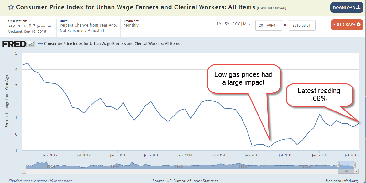
Does low inflation hurt investment?

It makes sense that a stable environment of low inflation should encourage business investment.  Low interest rates should encourage lending to business, etc.  This is the conventional narrative that has guided policy making at the Federal Reserve.  Stop an economist on the street and ask them if low interest rates encourage business investment and they will probably say yes. Here’s a quote from an economics course “If the expected rate of return [on the new investment] is greater than the real interest rate, the investment makes sense.”

Makes sense but what if it is partially wrong? Is it possible that low interest rates could, in some cases, discourage investment?  This is the opposite of the conventional narrative but let’s walk this path for a bit.  We often think of interest rates as a dependent variable, a response to something indicating a demand for money.  What if it is also an independent variable, a cause affecting the demand for money? Yep, it’s one of those interdependent cyclic things that might make you want to meditate on the universality of love and being, but stay with me 🙂

Interest rates can be a heuristic for investors, a signal of the demand for money, a weather vane of the underlying strength of the economy as seen by the top economists in the country, the folks at the Federal Reserve.  Low rates could be seen as a cautionary warning to investors.  If the economy were really getting stronger, would interest rates remain low?  Of course not, an investor might reason.  They would rise in response to stronger demand for money.  But they are not rising so better to be cautious, the investor reasons.  The dog chases its tail.

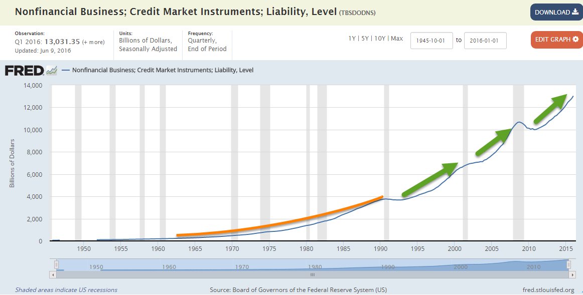
Do low interest rates cause reckless borrowing?

Are low interest rates prompting companies to borrow excessively?  Well, yes and no.  Yes, they are borrowing more but the growth trajectory, the rate of growth, is about the same as it has been since 1990.  As we can see in the chart below, each recession is a pause in the growth of corporate debt.  After each recession, the level rises again on approximately the same slope.  The “pause” in this last recession lasted a whopping four years, during which corporate debt declined as much as $600 billion, or about 5.6%.

The problem is what they are borrowing it for.  Companies typically buy back their own shares at their hghest, not lowest value.  By lowering the number of shares outstanding, buybacks raise the earnings per share even if there is no real growth in earnings.  Instead of buying low, selling high, companies tend to buy high, sell low. FactSet gathers and crunches a lot of market data.  Their mid-year analysis of share buybacks shows that total dollars spent on buybacks is approaching the highs of 2007.  Investment in real growth, in productive plants, equipment and office buildings, has declined the past three quarters but share buybacks, the appearance of growth, have increased.

A simple example

How could low inflation hurt investment?  If predicted inflation is rather low, about 2%, sales growth will not get that extra kick from inflation. Let’s say that a company’s sales are $1000 and the owners have an extra $50 to invest.  They are considering a plan to invest $50 and borrow $50 from the bank to expand in the hopes of making more sales.

First they consider the return by not expanding.  They put their $50 in the bank and make 2% interest or $1.  At 2% inflation, $1000 sales grows to $1020.  Let’s say that the company has a 30% gross margin, which gives an extra $6 profit on the extra $20 in sales.  The combined extra return to the owners is $7, a $6 profit and $1 in interest income.

Then they consider a second scenario.  Let’s say that the interest rate on the borrowed money is 6%, or 4% above the inflation rate of 2%.  As in the first scenario, they assume that the savings rate, or opportunity cost, of the invested $50 is about 2%.  The owners can expect an extra $4 imputed and actual cost on that combined $100 of investment.  If inflation is averaging 2% per year, then they can expect sales of $1020 even if there is no real sales growth.  Again, they use a 30% gross margin to arrive at an extra profit to them of $6, the same as the first scenario. If the extra investment does not produce any real sales growth, then the owners will net an extra profit of about $2, much less than the scenario of no expansion.  To make the same extra profit as in the first scenario, the owners need to generate an extra $11 in profit.  Minus the $4 in costs, the extra profit will be $7, the same as the first scenario.  Note that the owners are now trying to break even with the extra profits of not expanding.  To do that they must have sales of about $1037, or almost 2% real sales growth in addition to the 2% inflation growth.

Now, let’s consider a higher inflation rate of 4%.  Let’s imagine that the cost to borrow money is 8%, or 4% higher than inflation, as before, so that the cost of borrowing the $50 for a year is $4. As before, we’ll assume that the savings rate, or opportunity cost, of the $50 from the owner’ pockets is the same as inflation, or 4%, so that the imputed cost of the owners’ investment is $2.  Borrowed and imputed cost of the extra $100 invested in the company is now $6. If there is no real sales growth, total sales will now be $1040, or $40 more.  A 30% margin gives a gross profit of $12, leaving the owners with about $6 extra profit on investment.

Note that a doubling of the inflation rate in this scenario has produced a tripling of extra profit even with no real sales growth. Still the extra profits are less than not expanding at all.  They must still have a real increase in sales, but it is very small.

So a stable higher inflation rate and interest rate encourages business investment.  The key word here is stable.  We could keep doing this calculation with higher and higher rates producing more net profits to the owners but….  As inflation gets higher, it becomes less stable, less predictable and this unpredictability actually hurts business investment.

The Federal Reserve has set a target inflation rate of 2%.  I think it is too low and the lackluster growth of the economy seems to bear that out. Since the 1970s, prominent economists (Taylor and Tobin, for example) have suggested alternative targets that the Federal Reserve could use to replace the “dual mandate” set by the Congress in 1977.

A prominent alternative is a growth target in nominal GDP, called NGDP,  There are several variations but the one most favored has been level targeting, the calculation of GDP targets over the following five years or so based on an agreed growth rate.  The Fed would then take action to offset deviations from those targets. Two prominent economists, Robert Hall and Greg Mankiw, wrote a paper in 1993 explaining these alternative targets and the policy tools that the Federal Reserve could employ to help reach those targets.  During the period called the “Great Moderation,” from 1985-2007 national income grew at a rate just a bit more than 5%.

Hall and Mankiw noted (pg. 5) that the consensus among macroeconomists at that time was in favor of a targeting of nominal national income because it was a transparent measure, a clear, simple target.  The authors commented (pg. 4): “A rule like ‘Keep employment stable in the short run but prevent inflation in the long run’ [the current rule, by the way] has proven to be hopelessly vague; a central bank can rationalize almost any policy position with that rule.”

So the idea of nominal income or production targeting is familiar to economists and policymakers for several decades but has never been adopted. We can only assume, as the Nobel winner James Buchanan posited, that there is a very good reason for that.  When an obscure policy remains in place, it does so for a reason.  Enough policymakers want the obscurity that the policy provides.  I’m reminded of a letter John Adams wrote to Jefferson lamenting some of the vague language used in the Constitution which both of them had helped to craft.  Adams noted that the vagueness was necessary to reach consensus at the Constitutional Convention.  Efforts to achieve more precision in language or attempts to add specific detail were sometimes met with hardened disagreement.  The “general Welfare” wording of the tax and spending clause, Section 8, was one example.  Some argued that the lack of precision would give future generations of lawmakers some flexibility in determining what, in fact, was the general welfare of the United States.

 Whatever the Fed is doing now is only partially working and a different approach might be in order.  The use of the Labor Market Conditions Index, a broad composite of over twenty employment indicators, in guiding monetary policy shows that the Fed is reaching for a broader set of guidelines.  As Hall and Mankiw indicated, nominal targeting might give the Fed that broad guide, one that is less influenced by the needs and whims of elected politiciams.

Investment decline and the stock market

Let me finish on a somber note.  The year over year growth rate in the SP500 and private investment have both gone negative this year, for the first time since the end of the recession in 2009. The SP500 data is copyrighted so here’s a link to that chart. Pay attention.

/////////////////////////////

Notes:
If you would like to read more on the relationship of investment to savings, check out this 2006 NBER paper.

///////////////////////////

Happy Labor Day and put a shrimp on the barbie as a toast to the summer passing!

The Erosion of Inflation

August 13, 2016

What is inflation?  Commonly regarded as the change in prices from one year to the next, we can also define it as the rate at which the value of money declines.  In classical monetary theory, inflation reflects government demand for private savings.  When savings can not meet the demand, immoderate governments create the money they need.  This influx of invented money leads to higher prices and inflation.

Higher inflation encourages borrowers, including governments, since they can pay back loans borrowed in Year 1 with money that is worth less in Year 2.  A person who borrows $100 for a year at 10% interest but with 10% inflation, pays back a total of $110.  But the $110 is only worth 90%, or $99, in purchasing power.  In effect, the lender has paid the borrower for loaning the borrower money.  In a case like this, no one wants to lend money at that interest rate. The lender must charge a higher interest rate, driving up the price of borrowed money in a self-reinforcing tailspin of inflation chasing interest rates chasing inflation.

Deflation, or negative inflation, discourages borrowing for the opposite reason; money borrowed in Year 1 is paid back with money that is worth more in Year 2.  That same $100 borrowed for a year at 10% interest and 10% de-flation is paid back with $110 that now has the purchasing power of $121.  In this example, the borrower effectively pays the lender 21% interest.

I marked up a graph of post-1850 inflation I found here to show several key points in the “hockey stick” of inflation.

The Federal Government borrowed and spent a great deal of money during the Civil War period 1860-65, driving up the rate of inflation.   With a  currency backed by gold and sometimes silver, it took several decades of intermittent deflationary periods to correct for the imbalance of the Civil War.

When the Federal Reserve was created in 1913, the value of a dollar was little changed since 1850.  The Bureau of Labor Statistics doesn’t compile data on inflation before 1913.  After a World War and a severe short recession, a dollar in 1920 was worth half of what it was in  1913 {BLS }

Several years of deflation after the stock market crash restored some of the value to the dollar until the Federal Government began borrowing large sums of money to fund Roosevelt’s New Deal.  Inflation accelerated under the heavy government borrowing for World War 2.

Even though Roosevelt had ended the ready convertibility of dollars to gold during the Depression, several countries wanted cooperation in setting an international monetary standard.  At the Bretton Woods Conference in 1944, a year before the end of World War 2, the price of gold was fixed at $35 per ounce, a dollar benchmark that effectively made the U.S. dollar the world’s reserve currency.
In 1971, the Nixon administration removed that fixed price and allowed the dollar to float in price against gold and other currencies.  Within two years, the rest of the developed world followed suit.  A glance at the chart shows that this is the bend in the hockey stick, the point where cumulative inflation marches relentlessly upwards.

As I noted at the start, some inflation encourages borrowing. The keyword is “some.”  High inflation introduces so much uncertainty into the economy that it becomes debilitating.  Workers can not negotiate wage increases fast enough to keep up with the speed of inflation,, so they reduce their real spending.  Lenders demand high interest rates when they lend money in order to compensate for the declining value of money.  The high rates discourage borrowing and crimp economic activity.

A reasonable and fairly predictable inflation rate allows debt burdened governments to pay back borrowed money with money that has less value. In half a lifetime, from the point in 1973 when most governments freed their currency from a gold standard, the U.S. dollar has lost 80% of its value.  For the first two decades of these past forty years, family income kept pace with that loss of value.  During the last two decades the value of a family’s labor has been transferred to governments whose elected officials devise programs to return some of that transferred value to the most disadvantaged families.

In real terms, personal incomes have more than tripled since 1973 {Graph} but most of those gains were in the twenty-five years ending in 2000 when real personal incomes grew by 135%, a 5% annual pace.  In the sixteen years since 2000, real incomes have risen only 35%, averaging slightly above 2% per year.  When the value of money declines, the only way to save value is to invest money in assets, and only those on the upper half of the income scale have been able to preserve the value of their money in assets.  The lower half on that income scale has struggled.

As the value of money has declined in the past forty years, money invested in assets have gained in value. The press goes goo-goo as the SP500 makes new highs but that is a nominal value.  The inflation adjusted value is barely above its value in 2000 (Table) but has tripled in real value since 1973.  Home prices have not done as well but have gained 50% since 1975 (Graph).  For many families, their house is the majority of their assets and the inflation adjusted Case Shiller home price index is still below the level of ten years ago.

Elections are a competition of ideas for solutions and this election is no different.  The chief theme has been the ever declining value of money and labor, the relentless struggle of those on the lower half of the income scale. Folks on the political left favor ever more government intervention and clamor for more social programs to reduce household expenses, including free college tuition,  childcare and medical care. On the income side, the left calls for a doubling of the minimum wage.  Higher taxes and more debt will pay for these solutions.

Folks on the right side of the political aisle are ruled by an ideology that opposes government solutions, believing that there always exist remedies from the private sector even if there are no proposals for a private solution.  However, even those on the right want more government spending, but of the military kind, where it can most benefit families and economies in rural communities.  Donald Trump is now calling for greater infrastructure spending but this is sure to anger the conservatives in his party.  Folks on the right claim that more spending will be paid for by lower taxes on upper income families and the magic of wishful thinking called optimistic economic assumptions and dynamic budget scoring

For more than four decades, the world has been engaged in an international game of currency manipulation to prevent the fair market pricing of each country’s currency. Nations newly industrializing disregarded or gave a knowing wink to international agreements on labor practices and environmental protections.  Now the populations of the developed countries are aging and their birth rates are falling, particularly those countries in western Europe.  Already high government debt levels are strained by a swell of retiring workers who want the pension benefits they have been promised.  Economic growth that is sluggish or non-existent can not meet the demands for services and benefits, prompting more government borrowing.

Promises in a Presidential campaign are like unicorns.  After the election, the candidate removes the horn and voters realize that what they got was a rather good looking but ordinary horse, not a magical unicorn.  Promises are nevertheless calling cards to a political vision, and the vision of both campaigns is a rally ’round the flag of the domestic economy and American families. Trump’s supporters are endorsing his call for tariffs on imported goods to punish those countries which subsidize their industries and make American products less competitive in price.  Hillary Clinton is now calling for penalties for company inversions, the practice of relocating the legal presence of a business overseas to lower a company’s tax liability.  To rally their troops each candidate promises to fight the international system that threatens the well being of many American families.  However, it is our own government that is part of that system, the war on the value of money, on the value of work.

Pickup Purchasing Power

April 24, 2016

Relatively stagnant wages and income inequality have become a frequent theme on the campaign trail.  Let’s look at what I’ll call pickup purchasing power to understand the problem.  Sorry.  No graph from the Federal Reserve on this one.

A favorite vehicle among construction workers is the F-150 pickup, a reliable vehicle with room for a toolbox and a trip to the local lumberyard for supplies.  The MSRP of a standard bed 1998 model, available to the public in September 1997, was $14,835 (Source ) In 2016, the MSRP of that same model is $26,430 (Source), a 78% increase, about 3.2% per year.  There have certainly been improvements in that truck model in the past two decades but customers can not order the model without the improvements.  The basic model is the basic model.

Let’s look now at the wages needed to buy that pickup.  In May 1997, shortly before the 1998 F-150 was released to the public, the BLS survey reported average carpenters’ wages of $30,800.  At that time, wages and salaries were about 70.5% of total compensation, or about $43,700 (BLS report).  In the decade before that, wages as a percent of total compensation had declined from 73.3% in 1988 to 70.5% in 1997.  Rising insurance costs and other direct benefits to employees were slowly eating into the net compensation of the average carpenter.

In 2015, the average wage for carpenters was $43,530.  The BLS reported that wages were now 67.7% of the total employment cost, or about $64,300.  In that 18 year period, carpenters’ wages grew 41% but total compensation grew 47%, or 2.1% per year.  The price of that pickup truck, though, grew at 3.2% per year.  That seemingly small difference of 1% per year adds up to a big difference over the years.  That’s the sense of anger that underlies the current election season.  The growth in price of that pickup is only slightly above the average post WW2 inflation rate of 3%.  It is the wages that have fallen behind.

Trump blames the politicians who have given away American jobs with badly negotiated trade agreements that disadvantage Americans.  Trump’s promise to bring those manufacturing jobs back home wins him popular appeal in those communities impacted by the decline in manufacturing.  The loss of manufacturing jobs has left a larger pool of job applicants for construction jobs.  Some of those displaced workers did not have the carpentry skills needed but some were able to work in roles supervised by an experienced carpenter.  The more the supply of job applicants the less upward pressure on wages. If – a big if – some manufacturing jobs do come back to the U.S., it will help spur more growth in carpenter’s wages.

Bernie Sanders blames the fat cats and proposes taxing all but the poorest Americans to distribute income more evenly. His remedies to promote his programs of fairness are far ranging.  Employers who are currently providing health insurance for their employees will probably welcome a 6.2% payroll tax.  On a forty year old employee making $50,000 a year, the $3100 tax is far less cost than an HMO plan. Employers who do not provide such coverage will resent the imposition of more taxes but at least it will be across the board, affecting all competitors within an industry or local market.  Sanders’ healthcare plan also relies on 10% cuts in payments to doctors and hospitals, who are projected to save at least that much in reduced billing costs.

While Trump addresses a specific demographic, a particular segment of the labor market, Sanders proposes broad remedies to a number of problems.  Trump’s appeal will be to those who want a specific fix.  Bring back jobs to our community.  We’ll figure out the rest.  Sanders’ proposals will appeal to voters who have more confidence in government as a problem solver.

///////////////////////////

Oil Stocks

Readers who put some money to work in oil stocks (XLE, VDE for example) in late February, when I noted the historical bargain pricing, might have noticed the almost 20% increase in prices since then.  There are a number of reasons for the surge in price but the buying opportunity has faded with that surge.  Inventories are still high relative to demand.  Recent comprehensive market reports from the IEA require a subscription but last year’s report is available to those interested in a historical snapshot of the supply and demand trends throughout the world.  Until 2014, total demand had slightly exceeded supply.  A glance at the chart shows just how tightly coordinated supply and demand are in this global market. A “glut”in supply may be less than 1% of daily worldwide consumption and it is why prices can shift rather dramatically as traders try to guess both short and long term trends in demand and supply.

A Change Is Gonna Come

December 6, 2015

A horrible week for many families.  When we count the dead and injured in mass shootings, we often neglect to include the family and friends of each of these victims.  If we conservatively estimate 20 – 30 people affected for each victim, we can better appreciate the emotional and economic impact of these events. Shooting Tracker lists the daily mass shootings (involving four or more victims) in the U.S. in 2015.  What surprised me is that, in most cases, the shooter/assailant is unknown.

A strong November jobs report sent equities, gold and bonds soaring higher on Friday.  Markets reacted negatively on Thursday following a lackluster response from the European Central Bank(ECB) and comments by Fed chair Janet Yellen indicating that a small rate increase was in the cards at the mid-December Fed meeting.  The SP500 closed Thurday evening below November’s close.  Not just the close of November 2015, but also the monthly close of November 2014!

Overnight (early Friday morning in the U.S.), the ECB said that they would do whatever it took to support the European economy. Shortly after the cock crowed in Des Moines, the Bureau of Labor Statistics released November’s labor report, confirming an earlier ADP report of private job gains.  By the end of trading on Friday, the SP500 had jumped up 2%.  However, it  is important to step back and gain a longer term perspective.  The index is still slightly below February 2015’s close – and May’s close – and July’s close.

Extended periods of price stability – let’s call them EPPS – are infrequent.  Markets struggle constantly to find a balance of asset valuation. Optimists (bulls) pull on one end of the valuation rope.  Pessimists (bears) pull on the other end.  Every once or twice in a decade, neither bears nor bulls have a commanding influence and prices stabilize. Markets can go up or down after these leveling periods: 1976 (down), 1983 (up),  1994 (up), 2000 (down), 2007 (down), 2015 (?)

**************************

Year End Planning

Mutual funds must pass on their capital gains and losses to investors.  Investors who have mutual funds that are not in a tax-sheltered retirement account should take the time in early December to check on pending capital gains distributions either with their tax advisor or do it themselves.  Most mutual fund companies distribute gains in mid to late December.  Your mutual fund will have a list of pending December distributions on their web site.  For those retail investors in a rush, you might just scan through the list and look for those funds that have a distribution that is 5% or more of the value of the fund, then look and see if it is one of your funds.

An EPPS tends to produce relatively small capital gains but this year some mid-cap growth funds and international funds may be declaring gains of 7 – 10% of the value of the fund.  An investor who had $50,000 in some mid-cap growth fund might see a capital gain distribution of $4,000 on their December statement.  When an investor receives the statement in January 2016, it is too late to offset this gain with a loss.  Depending on the taxpayer’s marginal tax rate, they could be on the hook to the tax man for $700 – $1200.

Let’s say an investor is anticipating a $4000 capital gain distribution in a taxable mutual fund in late December.  Most mutual fund companies list the cost basis of each fund in an investor’s account. An investor who had a cost basis that was higher than the current value of the fund could sell some shares in that fund to offset some or all of the capital gain distribution in the other fund.  This is called tax loss harvesting.  Again, remind or ask your tax advisor if you are unclear on this.

Here is an IRS FAQ sheet on capital gains and losses.  Here is an article on the various combinations of short term and long term gains and losses.

**************************
CWPI

The latest ISM Survey of Purchasing Managers (PMI) showed that the manufacturing sector of the economy contracted in November.  October’s reading was neutral at 50.1.  November’s reading was 48.6.

The services sector, which is most of the economy, is still growing strongly.  Both new orders and employment are showing robust growth.   

However, manufacturing inventories have contracted for five months in a row.  For now, this decline is more than offset by inventory growth in the service industries.  However, the drag from the manufacturing sector is affecting the services sector.  The trough and peak pattern of growth in employment and new orders since the recession recovery in 2009 has begun to get a bit erratic.  Nothing to get too concerned about but something to watch.

The Constant Weighted Purchasing Index combines the manufacturing and service surveys and weights the various components, giving more weight to New Orders and Employment.  Both components anticipate future conditions a bit better than the equal weight methodology used by ISM, which conducts the surveys.  In addition, there is a smoothing calculation for the CWPI.

During this six year recovery, the CWPI has shown a wave-like pattern of growth.  Since the summer of 2014, growth has remained strong but there has been a leveling in the pattern as the manufacturing sector no longer contributes to the peaks of growth.

Despite the underlying growth fundamentals, there are some troubling signs.  In response to activist investors, to boost earnings numbers and maintain dividend levels, companies have bought back shares in their own company at an unprecedented level.  In some cases, companies are taking advantage of low interest rates to borrow money to make the share buybacks. (U.S. Now Spend More on Buybacks Than Factories, WSJ 5/27/15)

*******************************

Labor Report

46,000 jobs gained in construction was a highlight of November’s labor report and was about a fifth of all job gains.  Rarely do gains in construction outweigh gains in professional services or health care. This is more than twice the 21,000 average gains of the past year. The steady but slow growth in construction jobs is heartening but a long term perspective shows just how weak this sector is.

Involuntary part-timers, however, increased by more than 300,000 this past month, wiping out a quarter of the improvement over the past year.  These employees, who are working part time because they can not find full time work, have decreased by almost 800,000 over the past year.

The core work force, those aged 25-54, remains strong with annual growth above 1%.

Other notable negatives in this report are the lack of wage growth and hours worked.  Wage growth for all employees is a respectable 2.3% annual rate, but only 1.7% for production and non-supervisory employees.  This is below the core rate of inflation so that the income of ordinary workers is not keeping up with the increase in prices of the goods they buy.

Hours worked per week has declined one tenth of an hour in the past year, not heartening news at this point in what is supposed to be a recovery.  Overtime hours in the manufacturing sector has dropped 10% in the past year.

******************************

Inflation

The core CPI is a measure of inflation that excludes the more volatile price changes of food  and energy.  While the headline CPI gets the attention, this alternative measure is one that the Federal Reserve looks at to get a sense of the underlying inflationary forces in the economy.  The target annual rate that the Fed uses is 2%.

October’s annual rate was 1.9%.  November’s rate won’t be released till mid-December. However, Ms. Yellen made it pretty clear that the Fed will raise interest rates this month, the first time since the financial crisis. I suspect that prelimary reports to the Fed on November’s reading showed no decline in this core rate.  With employment gains and inflation stable, the FOMC probably felt comfortable with a small uptick in the bench mark rate.

Crossings

September 6, 2015

I am not going to say a lot about the August employment numbers, reported at 173,000,   since August’s numbers are routinely revised.  The BLS survey was 20,000 less than the ADP survey of private payrolls.  The revised figure will probably be closer to 210,000 jobs gained in August.  We can see the more important trends when we look at the annual job gains averaged over 12 months.

The slowdown in China and other markets and the selloff in markets around the world inevitably prompts talk of recession.  Since WW2 there has been only one recession – the one that followed the 1973 oil embargo –  that occurred when monthly job gains were above 200,000.   There have been 12 recessions since WW2. The work force was very much smaller fifty years ago.  There has been only one exception to this “rule” and when we look at this exception in closer detail we see that it was very much like the prelude to other recessions. Averaged monthly job gains were declining sharply as they do before every recession.  Job gains are NOT declining sharply today.

******************************

Resource Countries On Sale

Monday came the news that the Canadian economy was officially in recession.  California, the most populous of fifty U.S. states, has two million more people than all of Canada, whose economic vitality relies on its vast stores of timber, oil, gas and minerals.  Australia, Russia, Norway and New Zealand also ride the roller coaster of commodity prices. (WSJ article )  An ETF that captures a composite of Canadian stocks, EWC, is down almost 30% from its high of August 2014.  The 50 week (not day, but week) average is about to cross below the 200 week average.

These long term downward crossings are often bullish, indicating that prices are near a low point in the multi-year cycle.  An ETF composite of Australian stocks, EWA, is down a bit more than 30% and its 50 week average just crossed below the 200 week average.

A Vanguard ETF composite of energy stocks is near the lows of 2011.

********************
Subprime Mortgages

Conventional wisdom: subprime mortgages started the recent financial crisis in 2008.  A recent National Bureau of Economic Research (NBER) analysis (A short summary ) of home foreclosures overturns that misconception.  The authors found that twice as many prime borrowers lost their homes to foreclosure as subprime borrowers.

********************
Inflation

In 2007, the Social Security Administration estimated that prices would be 20% higher in 2015. Then came the severe recession of 2008-09 and persistently low inflation.  Prices this year are only 15% higher than those in 2007.  Social Security payments will total almost $900 billion this fiscal year (FRED series), more than 20% of Federal spending, and are indexed to inflation.  Low inflation “saves” the Federal government about $40 billion each year when compared with earlier projections.  Sounds good?  Life is a trade-off.  The 60 million (SSA) people who receive social security spend most of it.  That savings of $40 billion is money not spent.  In addition, low interest rates have reduced income for many retirees, who depend on safer investments for an income stream.  These safer accounts, which include savings, CDs, short and mid-term bond funds, have paid historically low interest rates since the Federal Reserve lowered its target interest rate to near-zero (ZIRP) in 2008.