Oh My Gawd!

November 8, 2015

There is the famous Tarzan yell by Carol Burnett and the iconic “Oh my Gawd” exclamation of Janice Lipman in the long running TV series “Friends.”  That’s what Janice would have said when October’s employment report was released this past Friday.

Highlights:

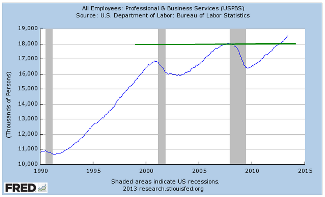
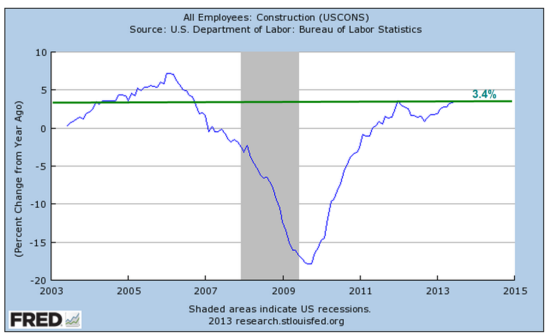
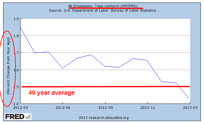
271,000 jobs gained – maybe. That was almost twice the number of job gains in September (137,000).  Really??!! ADP reported private job gains of 182,000.  Huge difference.  Job gains in government were only 3,000 so let’s use my favorite methodology, average the two and we get 228,000 jobs gained, awfully close to the average of the past twelve months.  Better than average gains in professional business services and construction.  Both of these categories pay well.  Good stuff.

At 34.5 hours, average hours worked per week has declined by 1/10th of an hour in the past year.  The average hourly rate rose 2.5%, faster than headline inflation and giving some hope that workers are finally gaining some pricing power in this recovery.

For some historical perspective, here is a chart of monthly hours worked from 1921 to 1942.  Most of those workers – our parents and grandparents – have passed away.  At the lows of the Great Depression people still worked more hours than we do today.  They were used to hard work.  There were few community resources and social insurance programs to rely on.

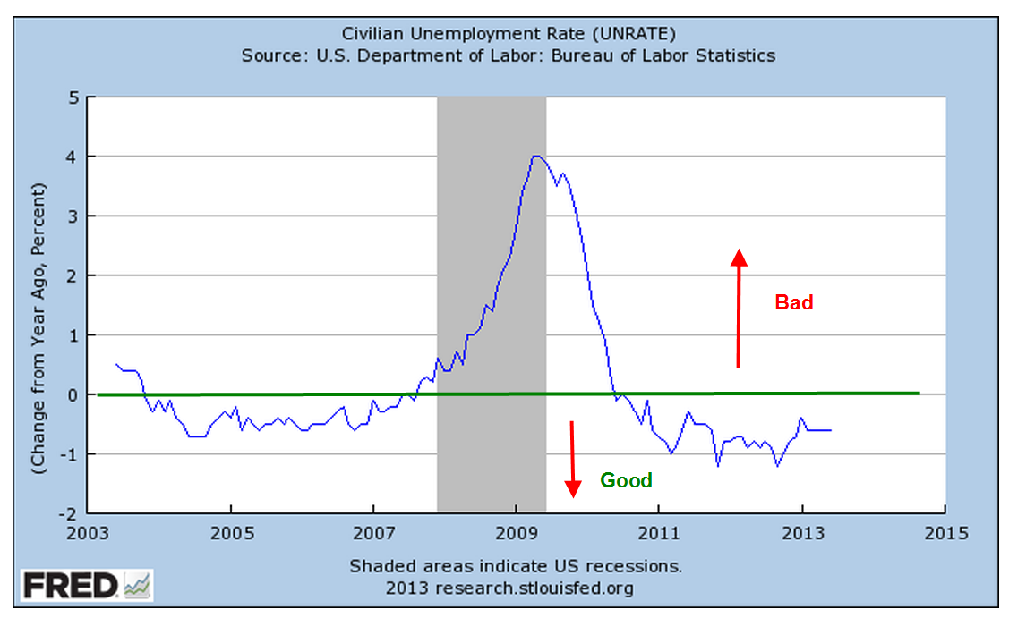
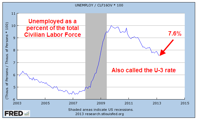
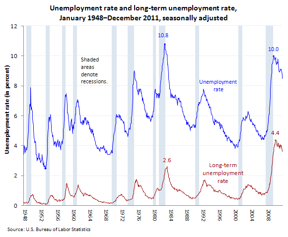
The headline unemployment rate fell slightly to 5%.  The widest unemployment rate, or U-6 rate, finally fell below 10% to 9.8%, a rate last seen in May 2008, more than seven years ago.  This rate includes people who are working part time because they can’t find a full time job (involuntary part-timers), and those people who have not actively looked for a job in the past month but do want a job (discouraged job seekers).  Macrotrends has an interactive chart showing the three common unemployment rates on the same chart.

The lack of wage growth during this recovery, coupled with rising home prices, may have made owning a home much less likely for first time buyers.  The historical average of new home buyers is 40%.  The National Assn of Realtors reported that the percentage is now 32%, almost at a 30 year low.

2.5% wage growth looks a bit more promising but the composite LMCI (Labor Market Conditions Index) compiled by the Federal Reserve stood at a perfect neutral reading of 0.0 in September.  The Fed will probably update the LMCI sometime next week.  This index uses more than twenty indicators to give the Fed an in-depth reading of the labor market.

**********************************

Bonds and Gold

The strong employment report increased the likelihood that the Fed will raise interest rates at their December meeting and this sent bond prices lower.  A key metric for a bond fund is its duration, which is the ratio of price change in response to a change in interest rates.  Shorter term bond funds have a smaller duration than longer term funds. A short term corporate bond index like Vanguard’s ETF BSV has a duration of 2.7, meaning that the price of the fund will decrease approximately 2.7% in response to a 1% increase in interest rates.  Vanguard’s long term bond ETF BLV has a duration of 14.8, meaning that it will lose about 15% in response to a 1% increase in rates.  In short, BLV is more sensitive than BSV to changes in interest rates. How much more sensitive?  The ratio of the durations – 14.7 / 2.7 = 5.4 meaning that the long term ETF is more than 5 times as sensitive as the short term ETF.

What do we get for this sensitivity, this higher risk exposure?  A higher reward in the form of higher interest rates, or yield.  After a 2.5% drop in the price of long term bond funds this week, BLV pays a yield close to 4% while BSV pays 1.1%.  The reward ratio of 4 / 1.1 = 3.6, less than the risk ratio.   On September 3rd, the reward ratio was much lower, approximately 3.27 / 1.3 = 2.5, or half the risk ratio.

Professional bond fund managers monitor these changing risk-reward ratios on a daily basis.  Retail investors who simply pull the ring for higher interest payments should be aware that not even lollipops at the dentist’s office are free.  Higher interest carries higher risk and duration is that measure of risk.

The prospect of higher interest rates has put gold on a downward trajectory with no parachute since mid-October.  A popular etf  GLD has lost 9% and this week broke below July’s weekly close to reach a yearly low.  Investors in gold last saw this price level in October 2009.  Back then  gold was continuing a multi-year climb that would take its price to nosebleed levels in August 2011, 70% above its current price level.

**********************************

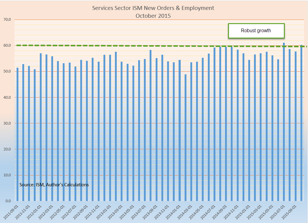
CWPI (Constant Weighted Purchasing Index)

Manufacturing is hovering at the neutral 50 mark in the ISM Purchasing Manager’s Index but the rest of the economy is experiencing even greater growth after a two month lull.  No doubt some of this growth is the normal pre-Christmas hiring and stocking of inventories in anticipation of the season.

The CWPI composite of manufacturing and service sector activity has drifted downward but is within a range indicating robust growth.

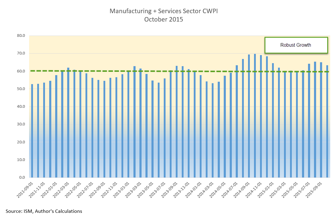
Employment and New Orders in the non-manufacturing sectors – most of the economy – rose up again to the second best of the recovery.

Economists have struggled to build a mathematical model that portrays and predicts the rather lackluster wage growth of this recovery in a labor market that has been growing pretty strongly for the past few years.

*************************************

Social Security

The Bipartisan Budget Act of 2015, passed and signed into law this past week, curtails or eliminates a Social Security claiming strategy that has become popular.  (Yahoo Finance – can pause the video and read the text below the video).  These were used by married couples who were both at full retirement age.  One partner collected spousal benefits while the “file and suspend” partner allowed their Social Security benefits to grow until the maximum at age 70.  On the right hand side of this blog is a link to a $40 per year “calculator” that helps people maximize their SS benefit.

************************************

Tax Cuts Anyone?

Former Senator, Presidential contender and actor Fred Thompson died this past week.  The WSJ ran a 2007 editorial by Thompson arguing that the “Bush tax cuts” that the Republican Congress passed in 2001 and 2003, when he was a Senator, had spurred the economy, causing tax revenues to increase, not decrease, as opponents of the tax cuts claimed.  Like others in the tax cut camp, Thompson looked at a rather small slice of time to support his claim: 2003 -2007.

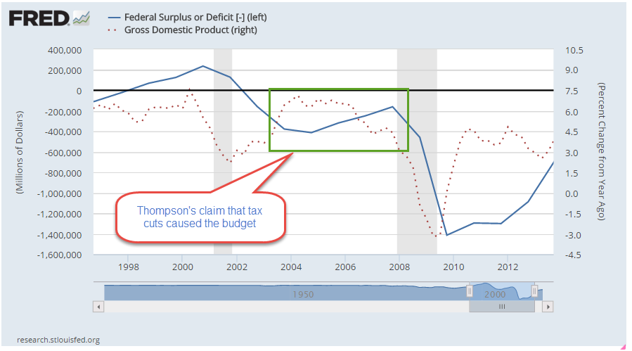
Had tax cut advocates looked at an earlier slice of time – also small – in the late 1990s they would have seen the opposite effect.  Higher tax rates in the 1990s caused greater economic growth and higher tax revenues to the government, thereby shrinking the deficit entirely and producing a surplus.

Tax cuts decrease revenues.  Tax increases increase revenues.  That tax cuts or increases as enacted have a material effect on the economy has been debated by leading economists around the world for forty years.  At the extremes – a 100% tax rate or a 0% tax rate – these will certainly have an effect on people’s behavior.  What is not so clear is that relatively small changes in tax rates have a discernible impact on revenues.  A hallmark of belief systems is that believers cling to their conclusions and find data to support those conclusions in the hopes that they can use that to help spread their beliefs to others.

The evidence shows that economic growth usually precedes tax revenue changes; that tax policy advocates in either camp have the cart before the horse.  A downturn in GDP growth is followed shortly by a decline in tax revenues.

Thompson’s editorial notes a favorite theme of tax cut advocates – that the “Kennedy” tax cuts, initiated into law in memory of President Kennedy several months after his assassination in November 1963, spurred the economy and increased tax revenues. Revenues did increase in 1964 but the passage of the tax act occurred during that year so there is little likelihood that the tax cuts had that immediate an effect.  Revenues in 1965 did increase but fell in subsequent years.  A small one year data point is all the support needed for the claims of a believer.

The question we might ask ourselves is why do tax policy and religion share some of the same characteristics?

Job Trends

July 7th, 2013
A better than expected June labor report released this week prompted some speculation that the Federal Reserve may begin tapering its quantitative easing program as early as this fall.  The employer survey reported a net gain of 195,000 jobs and the gains of earlier months were revised up 70,000.  Government workers continue to decline. We will see that the modest strength in the labor market is part of a mixed employment picture.    The unemployment rate remained steady at 7.6%; the year over year percent change in this headline index continues to chug along in the “good” territory.

70% of workers – about 95 million – are employed in private service jobs, most of which showed strong gains in the past quarter.

14% of workers are government employees; federal, local and state governments continue to shed workers.

As the number of workers declines, the number of people served by each worker continues to rise, approaching levels last seen in the early 1980s and mid-1970s.  The government work force would need to decline a further two million, or 10%, to reach the level of 15 people per government worker.  That level is still far below the comparatively lean government worker levels of the 1960s and earlier.

The major part of the attrition in government jobs seems to be over.  Local governments are adding employees while the federal government continues to shed employees.

Job gains continue to come in lower paying retail and food service jobs.  In 2013, employment finally surpassed early 2008 levels.  The average wage of $14 to $17 per hour in these industries is far below the $24 average of all workers and the $20 average of private production and non-supervisory workers.

Much higher paying jobs in Professional and Business Service industries continued to show strong gains and have also climbed above 2008 levels.  The average wage in this category is 15% higher than that of all workers.

Over seven million people not counted in the labor force or in the headline unemployment rate say they want a job now.  Four years after the official end of the recession, the number of “kind of unemployed” remains high.

The number of involuntary part-time workers increased by 322,000, or about 4%, to 8.2 million, over 5% of the total labor force.  These are workers who are working part time but want full time jobs.  A healthier labor market would have about 3% of these unwilling part timers.

As the number of housing starts increases, the unemployment rate among construction workers continues to decline and dipped below 10% this month.  Lower lows in this unseasonally adjusted index of unemployment is a good sign.

But the year-over-year percent change in construction employment is still not robust enough to reverse the heavy job losses since the onset of the recession.

The core work force aged 25 – 54 dropped by 100,000 and continues its slight upward struggle above the recession depths.

A decline in this prime working age population is partly responsible, but the 1.6 million decline in population is but a third of the 5 million plus decline in employment for this age group.

A 2004 paper by a BLS economist, Jessica Sincavage, provides an interesting historical perspective on multi-decade generational trends in the unemployment rate.  She noted “The characteristics of today’s younger workers differ from those of their baby-boomer counterparts in several ways that may affect the former group’s impact on the labor force and the unemployment rate now and in the future. Among the relevant characteristics affecting both groups are school enrollment patterns, race and Hispanic origin, and women’s labor force participation.”

In 1979, over 42% of the last of the boomer generation aged 20 – 24 were enrolled in school.  In 2002, under 37% of the “echo boomer” generation aged 20 -24 were enrolled.  Easy job availability, the growth of the internet and the sustained rise of the stock market during the 1990s persuaded many younger workers that the opportunity cost of going to college was simply not worth it.

The onset of this recession has divided the prime work force into two groups.  For those with a degree unemployment has remained low.  For those without the higher education, unemployment is almost double.  In a curious correlation, the unemployment rate for three groups is about the same – the general labor force,  workers above 25 years with a high school only education, and Hispanics.

The third factor noted by Ms. Sincavage is the participation rate of women in the labor force. In her 2004 paper she observed “In 1979, the participation rate of women 16 to 34 years was about 63 percent; by 1999, it was 70 percent.” By the mid 2000s, this cultural and demographic bulge began to decline.  The rate for all women has now declined below the levels of the early 1990s.

Although there was a lot to like about this month’s labor report, recent job gains are swimming against an undertow of shifting demographics and labor demands from employers.  A casual reading of the headline numbers might lead one to discount these long term negative trends.

Labor Participation Rate

April 6th, 2013

First I will look at a rather disappointing March Labor Report, released this past Friday.  Then I will zoom up and look at the big picture and some disturbing trends.  The net job gains this past month were 88,000, about half of the 169,000 average gains of the past year.  Remember that it takes about 150,000 job gains each month just to keep up with population growth.  Although the headline unemployment rate dropped .1% to 7.6%, it was because almost half a million people dropped out of the work force, meaning that they had stopped looking for a job in the past month.

Mitigating the meager job gains were revisions to previous months gains as more survey data was returned by employers. January’s job gains were revised from +119,000 to +148,000, and February’s gains were bumped upward from +236,000 to +268,000.  The two revisions added up to an additional 61,000 jobs; adding that to March’s gain of 88,000 gets close to the minimum gains needed of 150,000. The initial reaction of the market was a swift loss at Friday’s market opening of almost 200 points on the Dow.  By the end of the day, the market had regained much of the ground it lost, ending down about 40 points.

The average hours worked increased again to 34.6, a hopeful sign, but earnings saw no change.

Construction continued to show gains; the media’s attention to this area of employment probably gives the casual reader the impression that contruction jobs are a larger part of the work force than they actually are.

Compare that to Professional and Business Services, which has showed consistently strong gains and low unemployment.

Employment in the health care field continues to grow.  As a percent of total employment, health care continues to reach new heights, although its growth has moderated.  Taking care of the sick may be a sign of a compassionate society, but it consumes resources, prompting the question: what is the upper limit?  One in nine workers now work in health care.  Twenty years ago, the ratio was one in twelve. 

Over the past twenty years, the employment market has shifted markedly away from producing goods.  As a share of total employment, about 1 in 7 workers produces goods.  Just ten years ago, the ratio was 1 in 6.

What jobs did those workers find?  Serving food and drink to the ever growing share of people in Professional and Business Services.

The core work force, those aged 25 – 54, shows no growth over the past year.  I use the words “work force” to include only the employed.  “Labor force” includes both the employed and unemployed.  More on that in a bit.

I have written before about the year over year (y-o-y) percent change in the headline unemployment rate, or U-3 rate, and that past recessions usually follow when this change goes above 0.  The unemployment rate has benefitted remarkably from the number of people who continue to drop out and are no longer counted as unemployed.  Because of the drop outs the percent change in the unemployment rate is still in good territory.

A secondary indicator may be the y-o-y percent gain in the employed.  The long term average is 1.5%.  When the percent gain falls below that, recession soon follows.  The percent gain just fell below the long term 1.5% average.

Let’s zoom out to the past forty years to see how this percent gain in employment has preceded past recessions.  The exception was in 1973-74 when the Arab oil embargo created a sudden and deep recession in the country.

There was a decline in the number of people who dropped out but had been searching for work (but not in the past month) and were available to work.

The long term trend of those not in the labor force continues to reach new heights.  As a percent of the population, it  keeps climbing at an alarming rate.

Older workers are retiring, either voluntarily or involuntarily, at the rate of 800,000 a year.

Which brings us to several sometimes confusing concepts, the Civilian Labor Force (CLF), the Participation Rate, and other metrics.  The Civilian Labor Force is those people aged 16 and over who are either employed or unemployed.  To be counted as unemployed, a person is not working but has searched for work in the past month.  The unemployment rate is simply the percentage of unemployed in the Civilian Labor Force, which now totals about 155 million.  An unemployment rate of 7.6% means that about 12 million people are counted as unemployed. 

Then there is the Civilian Labor Force Participation Rate, or simply the Participation Rate, which is the percentage of the Labor Force to what the BLS calls the Civilian Non-Institutional Population (CNP).  Don’t go to sleep on me.  The CNP is those people who are aged 16 or more and who are not in prison or the military. 

So, the Participation Rate (PR) is the number of people who ARE working as a percent of people who CAN legally work; i.e. who are over 16 and not in some institutional setting that prevents them from working or finding work.


Let me give you some numbers and a pie chart.

The total population of the U.S. is estimated at 313 million; the CNP is estimated at 245 million.  The difference between those two figures are mostly children under 16 and people in prison and the military.  Here’s how the Labor Force compares with those not in the labor force and children under 16.

Why does the the Participation Rate (PR) matter?  As it declines, workers have to support more of those who are not working.  Many seniors feel that they “paid into the system” but the “system” – yes, your elected representatives in Congress – spent the additional money paid into the system over the past thirty years.  Social Security is a “Pay as you Go” system meaning that existing workers must somehow pay back into the system to pay benefits for those who retire.  Pay back = higher taxes. As the percentage of the population who works declines, taxes must rise or benefits decrease regardless of who paid into the system. 

This past month the BLS estimated a further decline of .2% to a level of 63.3%.  For comparison, Canada has a PR of 66.6%. 

Part of the decline is a natural demographic change as the population ages.   So how much has the aging of the population contributed to the decline in the PR?  What is the PR for those of working age 16 – 64?  Oddly enough, the time series figures are not easy to come by.  But before we get to that, let’s get to the surprises.

Since 2010, the older labor force, those aged 65+, has grown by 1.2 million. 

In 20 years, the participation rate among seniors has risen 50%, from 11.8% in 1990 to 17.4% in 2010.  The BLS projects that it will rise to 22.6% by 2020, a doubling in thirty years.  Seniors will continue to compete for jobs with the working age population.

Meanwhile, the participation rate of the core work force, those aged 25 – 54, is on a steady decline.

Now comes the biggest surprise, the decline in the working age Participation Rate.  To get the time series, I had to add a number of series together and take some population estimates by the Census Bureau.  Changing demographic shifts and 2010 census revisions make the series not entirely accurate but does give a good representation of the approximate 6% decline.

Let’s look at the last five years for the overall Participation Rate, which has declined about 5%. 

The aging of the population is contributing maybe 20% to the overall decline.  The bulk of the decline is a deterioration of the working age labor force.  Some are going back to school, some have given up looking for a job recently.  Many younger workers are finding it difficult to find a job. The Consumer Credit report released Friday shows another surge in student loans.  The FinAid student debt clock shows that student loans now exceed a trillion dollars. I have the sinking feeling that this will end badly. The participation rate for those aged 20 – 24 has declined about 7% and is now slightly less than the rate for all working ages. 

Payments under the Social Security Disability program, or SSDI, took about 10% of Social Security taxes in 1984.  They now consume 20% of SS taxes and are becoming an increasing burden on the Social Security program even as the boomers begin to retire.  The ranks of the disabled have grown more than 10% in the past three years.

A declining percentage of the population working to pay for an increasing number of benefits – this economic tension is sure to produce social and political conflict.  Many of us probably hold the vague hope that it will all work out somehow.  Some think that politicians in Washington will figure it out despite the fact that the solutions that Congress comes up with to most problems only exacerbate the problem or shift the problem to another area.

On the other hand, the baseball season is still young and anything is possible, right? 

Labor Report – July

Skipping into the Oval Office Friday morning, President Obama’s campaign manager called out with glee, “Mr. President, 163,000 jobs!”
“Buy, buy, buy!” traders shouted on the floor of the N.Y. Stock Exchange.
“Let’s take a six week vacation!” John Boehner, the House Speaker, cried out.
Concentrating on the .1% uptick in the unemployment rate, Presidential contender Mitt Romney said, “the president’s policies are to blame for not having gotten the economy back on track.”

What to make of these conflicting numbers?  Economists and market watchers were anticipating a gain of 100,000 jobs.  Economists guesstimate that a growth of 150,000 jobs per month is needed to absorb the increase in the working population.  163,000 is above 150,000; so how did the unemployment rate tick up from 8.2% to 8.3%?

The headline job gain number comes from the Current Employment Statistics program, a monthly survey of 141,000 businesses and government agencies that represent almost a half million worksites.  This “Establishment Survey”, as it is sometimes called, counts jobs, not people.  The addition of two part time jobs will count as two jobs even if only one person is working those two part time jobs.  Not all businesses return their survey forms to meet the monthly deadline so the Bureau of Labor Statistics (BLS) estimates the results and this first estimate becomes the headline number that gets so much attention from the market and political pundits.  The following month the BLS issues a 2nd estimate, followed by a 3rd estimate a month later.  The chart below shows the differences between the 3rd estimate and the first estimate (BLS source ).  As you can see, the revisions can be substantial. (Click on graphs to open in a separate tab)

On September 2nd, 2011, the BLS released their August report showing a gain of 0 (zero!) jobs.  The stock market sank 2.6%.  The 3rd estimate, released in November, showed job gains of 104,000, not 0!  The BLS will further revise the job gains for a particular month as state unemployment reports and other data becomes available to the BLS.

These job gains are seasonally adjusted.  One of the seasonal adjustments for July is the customary shut down of auto factories in July.  This year, in response to demand, auto manufacturers did not shut down their factories but the BLS makes the adjustment regardless.  Several analysts reason that this seasonal adjustment accounted for about 25,000 of the 163,000 jobs gained.  Despite all these shortcomings, the CES is regarded as the more accurate count of jobs.

The unemployment number comes from a separate monthly survey of 60,000 households conducted by the BLS.  While the Establishment Survey does survey small businesses, it misses a good chunk of the really small businesses, the mom and pop operations, that form an important backbone of the economy.  The Household Survey is often thought to overestimate the total number of jobs in the economy but it gives a detailed picture of the workforce and the unemployed.  From this survey we learn of the age, racial, and education characteristics of the employed.  Each month I look at two aspects of this survey: the growth or decline in what I call the core work force, those aged 25 – 54 years old, and the larger workforce aged 25 and older.  The actual number doesn’t matter as much as the increase or decrease in the adult work force – the trend in job growth.

The graph below charts the year over year percent gain or loss in the core work force.  It is still positive, leveling off after climbing up from negative territory a year ago.

For a bit more perspective, let’s zoom out and look at the past 20 years.

A graph of the year over year percentage gains in the larger work force aged 25+ shows that we have just about reached the high point of job growth during the 2000s.  We would need to at least maintain this level of growth to make up for the job losses during this past recession.  We would like to see job growth more like those we experienced during the high tech boom of the 1990s but the investment in new technology during the 1990s was particularly strong.  A catalyst for such a fundamental growth in the economy is not on the horizon.

The market experienced what I think is a relief rally on Friday.  Persistent troubles in Europe, a slowdown in the growth of China and other Asian emerging economies, lackluster employment reports for May and June, and a tepid 1.5% GDP growth in the second quarter had spread fears of a coming double dip recession. Had the BLS issued a job gains estimate of 50,000, for example, the market would have probably declined 2+%.  Back in April of this year, I wrote about an employment indicator that has been a reliable predictor of recessions.  When the percent change in the unemployment level crosses above zero percent, it’s time to get into the storm cellar and batten down the hatches!

-1% is an indicator of a rebounding labor force midway in a recovery from a recession.  I’ve marked up a thirty year chart of the year on year (y-o-y) percent increase/decrease in the unemployment rate to show the trend.  Had we not shipped so many jobs to China after they joined the World Trade Organization in 2001, we might have had the spurt of job growth recovery that we experienced in the early eighties. 

As the chart below shows, that kind of strong post-recession job growth is not the norm.

Larry Kudlow, a CNBC host, and other “supply sider” pundits are presently making the case that Presidential contender Mitt Romney will usher in a new era of the same kind of unusual job growth we experienced in the 1980s.  Anything is possible, of course, and hosts of financial shows make their money by making headline predictions.  Those of us without a TV show must pay more diligent attention to the law of averages, to the probable, not the possible. That law of averages makes it unlikely that either a President Obama or a President Romney will achieve historically unusual declines in unemployment.  In Britain the slow news months of summer are called the “silly season”.  In these few months before the election, Americans will experience a truly silly season, not for the slowness of news but for the sheer deluge of outlandish and annoying political ads making accusations and far-fetched claims. After that silly season will come another silly season, the Christmas shopping tournament! 

May Labor Report

May’s monthly Labor Report headlined a seasonally adjusted job gain of about 70K, less than half of the 150K expected.  The stock market response was swift and worsened as the day’s trading progressed.  By the time the dust cleared Friday evening, the broader S&P500 index had lost about 2.5%, it’s worst daily performance since Oct. 3, 2011.

On Feb. 5th, I wrote in response to the January labor report showing a gain of 234,000 jobs: “With the S&P500 index at 1344, some market pundits are whispering the 1500 mark that the S&P could take a run at this year.  Holy moly, macanoli, what a buzz about one labor report!” and later “Any job growth is good, but when I see a better improvement in the employment numbers for [the core work force aged 25 – 54], I will know that we are building a resilient economy, one that can withstand some shocks.”

Remember, the headline numbers are seasonally adjusted.  For the past three years, market watchers and economists have been warning about the seasonal adjustment factors used by the Labor Dept.  The severe job losses in the fall and winter of 2008/2009 have probably skewed the adjustment factors, leading the Labor Dept to overstate job gains during the winter and understate job gains in the spring and summer months.  The unusually warm winter of 2011/2012 further skewed job gains, pushing some normal spring hiring forward into the winter months.  That’s why I look at year over year gains in unseasonally adjusted numbers, particularly in the core work force aged 25 – 54.

Below is a graph of the percent gains of the core work force, which accounts for about 2/3 of the total work force.  The FED has conveniently saved me the trouble of running the graphs from the Labor Dept – but mine are more colorful :-).

The headline numbers of monthly job gains of more than 200K led many investors to bid up stock prices a bit more than the job gains in the core work force warranted.  Friday’s stock market reaction was probably a bit much but many investors simply bailed.  The same stock price and labor market patterns of 2010 and 2011 are emerging again this year.  Last June, I wrote about a backtest of investing based on the old “Sell In May and Go Away” mantra. While that investment strategy underperformed regular monthly investing, it has been disturbingly profitable for the past two years and looks to repeat again this year.  The disappointing labor figures only compounded the worries about the ongoing recession and financial woes in Europe, causing many to bail out of the market.

Let’s “zoom out” on the core work force, looking at the past year and a half.  There is a definite positive trend in place.

Let’s fly up like little birdies and look at the core work force for the past 12 years to see this recent upward trend in perspective.

Let’s look at the larger work force, those aged 25+, which accounts for 88% of employment in this country.  The year over year gains have leveled off at about 1.6% in the past few months.

Looking back the past 12 years, we see that this gain is moderately healthy.  The housing bubble produced employment gains of over 2% – gains concentrated in construction.

Now let’s look back to the “roaring nineties,” before China joined the WTO in 2001, leading to a loss of 4 million manufacturing jobs in this country.  The country enjoyed a tech boom in that decade, eventually leading to the dot-com bubble as we approached the millennium mark.

The job gains these past 6 – 8 months are respectable, averaging what they were in the nineties; core work force numbers are still growing.  The job losses of this past recession were historic.  Most of the 8.13 million jobs lost happened before Obama took office and the job losses were staggering when compared to other recessions.  The 1982-84 recession, for comparison, suffered total job losses of 2.84 million, about a third of the job losses of this past recession. Below is a graph of the year over change in employment levels since 1948.  This past recession makes all the past recessions look like small wrinkles.  Job losses of this size severely weakened the structure of our economy.

The employment growth of the past few years has been respectable, even more so given the deep hole our economy is climbing out of.  We are a people who have become accustomed to instant gratification.  We want change and we want it now, dammit.  The political and media machines of both parties know this and play to it.  George Bush played to it in the 2000 campaign, promising to bring the parties closer together, only to drive them further apart.  Obama played to it in his 2008 run for the White House, promising to usher in a new era of honest and accessible government, of community of government and the middle classes, where everyone enjoyed a more even playing field.  Romney’s run for the Presidency will highlight his business experience, promising unspecified growth policies.  What all of these people and their advisors know is that the American public is a sucker for change, reaching for the brass ring of change as we whirl around on the political merry-go-round.  We can be easily lied to because we trust our guts, not our brains.  If we trust someone or agree with their ideology, we will believe almost any data they throw at us.  Most of us don’t check the data.  We’re too busy for that or we don’t know how to check the data.  It all becomes a blur of he said this and the other guy said that and we get confused and vote with our guts.  The parties play to our prejudices.  Think you don’t have any?  Think again.

This election season we will hear a lot of claims, accusations and refutations.  Moderators of the upcoming Presidential debates rarely challenge a candidate with data.  The moderators ask policy questions; the candidate responds with mostly rehearsed answers.  Then on to the next question.  It is up to us to do our homework but most of us won’t.  Too many of us may be like the caller to a talk show recently.  When confronted with government statistics that refuted the caller’s opinion, he responded “That can’t be right” and countered that the government data is wrong.  We do love our opinions and that is the number one prejudice we all share. 

Labor Report – February

This past Friday, the Bureau of Labor Statistics (BLS) released their monthly assessment of the labor market, reporting a net increase of 227,000 jobs during the month of February.  This marked the third consecutive monthly increase of more than 200,000 jobs, giving many hope that the tepid economic recovery is gaining a firmer foothold.  Consumer spending accounts for more than 2/3 of the economy.  Any improvements in the overall economy are fragile without a strengthening labor market.  Almost 1/2 million people who had previously given up looking for work became available for work again.  This influx of job seekers offset the rise in jobs, causing the unemployment rate to remain unchanged at 8.3%.

The monthly survey of businesses showed job gains in many industries:  Business services, leisure and hospitality, health care, mining and manufacturing. In 2011, government jobs disappeared at the rate of 22,000 per month.  That job attrition has slowed to zero, indicating that the cut backs in government are largely over and will no longer weigh down any growth in the private sector.

The bad news is that there are many critical elements of the jobs report that were unchanged.  The long term unemployed remained about the same at 5.4 million.  The participation rate of the 155 million civilian labor force is a bit less than what it was a year ago but the employment population ratio is slightly above Feb. 2011’s rate.  The average workweek remained unchanged at 34.5 hours.  Involuntary part time workers, those who would like a full time job but can’t find one, remained the same at 8.1 million. 

As encouraging as February’s data is, the 5.4 million who have been unemployed for 27 weeks or more is a troubling sign of the underlying weakness of the job market.  Below is a BLS historical comparison of the unemployment rate and the long term unemployment rate.  The 70 year timeline of the graph illustrates the ongoing crisis levels of long term unemployment.

On Monday, March 12th, the BLS will release the monthly JOLTS job openings report for January 2012.  In December, there were 3.4 million seasonally adjusted job openings, an increase of almost 10% from the previous month.  This is better but – always that but – the graph below shows non-seasonally adjusted (NSA) December job openings from the previous ten years to show the improving but still weak number of job openings.

As I have mentioned in past blog posts, there is some concern that the seasonal adjustments that the BLS uses may have some weaknesses due to the severe downturn in the fall of 2008 which affected the winter seasonal adjustments.  The BLS makes one set of seasonal adjustments for the six months from May through October and another set of adjustments for the November through April period.  With advances in statistical modeling that the Census Bureau has introduced over the past 50 years, the BLS has refined their methodology of making seasonal adjustments.  The concern is not with their methodology but with the data itself of late 2008 and early 2009, an “outlier” that was so extreme that it “contaminates” the data set in subsequent years. The BLS incorporates 5 years of data in their projections of seasonal adjustments, so this “hangover” will last into the spring of 2014.  You can read an overview of the adjustment methodology used by the BLS here.  Without seasonal monthly adjustments, January’s job data each year would look dismal, with job losses regularly in the 2.5 to 3 million range, as employers lay off workers who were hired for the Christmas season.

A comparison of the raw numbers for job gains in February of each year do give an indication of labor market momentum.  As the chart below shows, the gains in February have been one of the strongest of the past decade.

But we saw strong gains last year throughout the spring only to see the momentum fade, explaining why the reaction to this month’s gains have been one of “cautious optimism”.  Some attribute the loss of momentum last year to the tsunami, the unrest of the Arab spring and rising gas prices, the ongoing sovereign debt problems in Europe, and the embarrassing budget battle.  But there may be more to it than the events of last year.  I contend that there is a structural weakness in our labor market that makes us more susceptible to the “winds” of current events.

As I have done before, let’s look at the core working population, 25 – 54 years old.  These are non-seasonally adjusted figures for February in each of the past ten years.

These are the “middlers”, those of us who are buying homes for the first time, raising families, buying appliances and cars and they are the backbone of a consumer economy.  The job growth of this population backbone has been flat and remains at levels below those of the early part of the decade, as this country pulled out of the 2001 – 2003 downturn.

The largest part of the increase in employment have come from those who are older than 54, as shown in the chart below of the larger data set of those 25 and older who are employed. Partially this is due to an aging population – the graying of the Boomers – but it shows a structural weakness in the labor market which undercuts the resilience of the economic recovery.

The takeaway is that we are once again seeing improvement but our economy and labor force suffers from a brittleness that the labor data exposes.  Part of that brittleness is due to an aging population; part is due to the continued de-leveraging and slow recovery typical of major financial crises; part is due to political indecision in government which reflects the indecision and disagreement among the voters; part is due to a very “accommodating” (translation: low interest rates) Federal Reserve policy that attempts to distribute financial pain, reward and risk throughout the economy using the few monetary tools that it has.

The stock market is encouraged but stuck. After rising for the past two years, the 200 day moving average of the SP500 has leveled off for the past 6 months, a phenomenon not seen since April to October of 1994.  October 1971 to March 1972 and May through September 1957 saw a similar 6 month plateau.  The Indians in the market are hunched over with their ears to the ground, not certain whether the distant sounds they hear are buffalo or thunderstorms.