Profits and Savings Diverge

November 20, 2022

by Stephen Stofka

This week’s letter is about household savings and corporate profits. As a share of GDP, savings are near an all-time low while profits are at an all-time high. Elon Musk, the CEO of Tesla, appeared in court this week. No, this wasn’t about his acquisition of Twitter. It concerned a shareholder lawsuit against Tesla regarding the $50B stock option package the company awarded him in 2018. In 2019 the company’s total revenue – not profit – was less than $25B. In 2022, annual revenue was $75B. At a 15% profit margin, the company must continue growing its revenue at a blistering pace to afford Mr. Musk’s incentive pay package. Large compensation packages like this are only a few decades old. Let’s get in our time machine.

In 1994, Kurt Cobain, the 27 year old leader of the rock group Nirvana, died from an overdose of heroin. Something else was dying that year – corporations were breaking free of national boundaries and moving production to countries other than their home nation. This was the last stage in the evolution of multinational corporations, or MNCs. In earlier decades, companies had licensed or franchised their brand. Perhaps they had set up a sales office in a foreign country. Now they were becoming truly global. Fueling that expansion was an increase in equity ownership by large institutional investors. To accommodate these changes, their governance structures changed. Executives capable of leading this global growth were rewarded on a parallel with superstar sports talent. That was the conclusion of Hall and Liebman (2000, 3), two researchers at the National Bureau of Economic Research. 

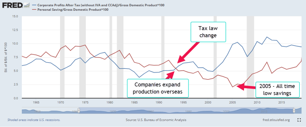
Let’s look at two series over the past sixty years – personal savings and corporate profits. If we think of a household as a small enterprise, personal savings is the residual left over from the household’s labor. Likewise, corporate profits are the residual left over from current production. In 1994, the two series diverged. Corporate profits (the blue line in the graph below) kept rising while personal savings plateaued for a decade. Each series is a percent of GDP to demonstrate the trend more easily.

Executive Compensation

In the mid-1990s, corporations began to issue a lot more stock options to their executives. Some think that a change in the tax code might have precipitated this shift in compensation.  In 1994, Section 162m of the IRS code limited the corporate deductibility of executive pay to $1 million (McLoughlin & Aizen, 2018). By awarding non-qualified stock options to their executives, companies could preserve the corporate tax deduction. However, the slight tax advantage did not account for the rapid increase in options awards. Hall and Liebman found that the median executive received no stock option package in 1985. By 1994, most did. The tax change was secondary – a distraction. Institutional investors wanted more growth and more profits and companies were willing to reward executives with compensation packages similar to sports stars (Hall & Liebman, 2000, 5). Some of these superstars included Jack Welch of General Electric,  Bill Gates of Microsoft, Michael Armstrong of AT&T.

Income Taxes – Less Savings

In 1993, Congress passed the Deficit Reduction Act that raised the top tax rate from 31% to almost 40%. Personal income tax receipts almost doubled from $545 billion in 1994 to almost $1 trillion in 2001. The booming stock market in the late 1990s produced big capital gains and taxes on those gains. For the first time in decades the federal government had a budget surplus. However, more taxes equals less personal savings so this contributed to the flatlining of personal savings during that period.

Household Debt Supports More Spending

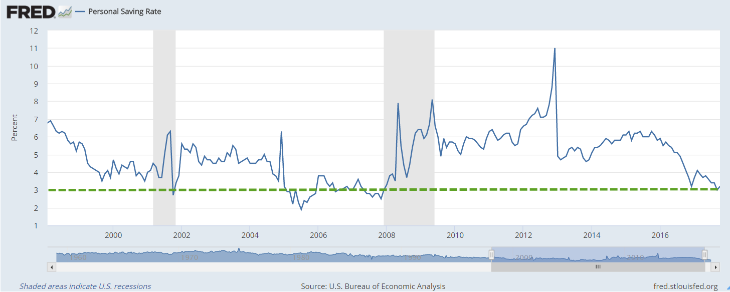
During the 2000s, personal savings remained flat. On an inflation adjusted basis, they were falling. Too many people were tapping the rising equity in their home to pay expenses and economists warned that household debt to income ratios were too high. Savings as a percent of GDP fell to a post-WW2 low. As home prices faltered and job losses mounted in late 2007, people began to save more but their debt left them with little protection against the economic downturn. During 2008, personal savings began to increase for the first time in fifteen years. More savings meant less spending, furthering the economic malaise that began in late 2007.

Multi-National Corporate Profits

During those 15 years corporate profits rose steadily as companies increased their global presence. Beginning in 1994 U.S. companies began shifting production to Mexico where labor was cheaper. In 2001, China was admitted to the World Trade Organization (WTO) and production outsourcing continued to Asia. Despite the profit gains, companies kept their income taxes in check. In 2021, corporate income taxes were at about the same level as in 2004. That contributed to the rising budget deficit during the first two decades of this century.

Federal Deficit

The prolonged downturn in 2001-2003 and the financial crisis and recession of 2007-2009 put a lot of people out of work. This triggered what are called “automatic stabilizers,” unemployment insurance and social benefits like Medicaid, housing and food assistance. The federal government went into debt to pay for the Iraq War, pay benefits to people and help fill the budget gaps in state and local budgets. The tax cuts of 2003 enacted under a Republican trifecta* of government control reduced tax revenues, further increasing the deficit. During George Bush’s two terms, the debt almost doubled from $5.7 trillion to $11.1 trillion.

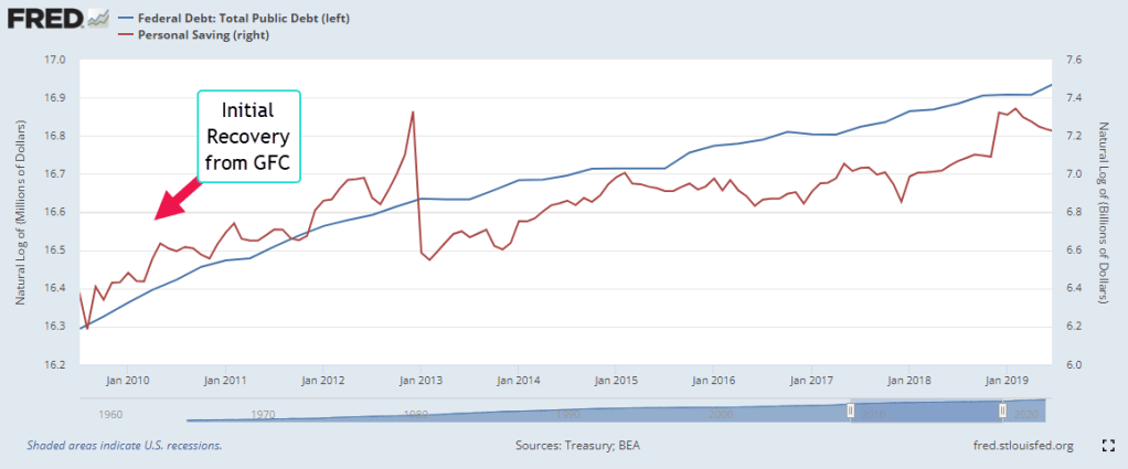
In coping with the recovery from the financial crisis, the government added another $8.7 trillion to the debt. That negative saving by the government helped add to the personal savings of households but too much was spent on just getting by. Following the Great Financial Crisis (GFC), the trend of the government’s rising debt (blue line below) matched the trend in personal savings (red). Sluggish growth and lower tax revenues caused the two to diverge. While the debt grew, personal savings lagged.  

Before and During the Pandemic

Following the 2017 tax cuts enacted under another Republican trifecta, personal saving rose, then spiked when the economy shut down during the pandemic and the federal government sent stimulus checks under the 2020 Cares Act. In the chart below, notice the spike in debt and savings. By the last quarter of 2020, personal savings had risen by $600 billion from their pre-pandemic level of $1.8 trillion. In late December, President Trump signed the $900 billion Consolidated Appropriations Act (Alpert, 2022) but that stimulus did not show up in personal savings until the first quarter of 2021. In March 2021 President Biden signed the $1.7 trillion American Rescue Plan. Personal savings rose $1.6 trillion in that first quarter, the result of both programs.

After the Pandemic

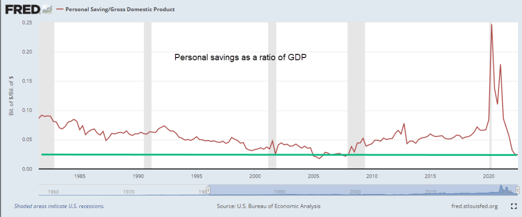
Some economists have said that the American Rescue Plan was too much. In hindsight, it may have been but we don’t make decisions in hindsight. As more schools and businesses opened up, households spent far more than any extra stimulus. They spent $1.2 trillion of savings they had accumulated before the pandemic and savings are now at the same level as the last quarter of 2008 when the financial crisis struck. Thirteen years of cautious savings behavior has vanished in a few years. On an inflation-adjusted basis, personal savings is at a crisis, almost as low as it was in 2005. In the chart below is personal savings as a ratio of GDP.

The Future

In the past year savings (red line) and corporate profits (blue line) have resumed the divergence that began almost three decades ago. Profits were 12% of GDP in the 2nd quarter of 2022. Savings is near that all time low of 2005. Rising profits benefit those of us who own stocks in our mutual funds and retirement plans. However, the divergence between the profit share and the savings share is a sign that the gap between the haves and the have-nots will grow larger.

////////////////////

Photo by Jens Lelie on Unsplash

  • A trifecta is when one party controls the Presidency and both chambers of Congress.

Alpert, G. (2022, September 15). U.S. covid-19 stimulus and relief. Investopedia. Retrieved November 19, 2022, from https://www.investopedia.com/government-stimulus-efforts-to-fight-the-covid-19-crisis-4799723. See Stimulus and Relief Package 4 for the December 2020 CAA stimulus. See Stimulus and Relief Package 5 for the American Rescue Plan in March 2021.

Hall, B. J., & Liebman, J. B. (2000, January). The Taxation of Executive Compensation – NBER. National Bureau of Economic Research. Retrieved November 19, 2022, from https://www.nber.org/system/files/chapters/c10845/c10845.pdf. Interested readers can see Moylan (2008) below for a short primer on the recording of options in the national accounts. Until 2005, these options were recorded as compensation for tax purposes but not recorded on financial statements so they did not initially affect stated company profits.

McLoughlin, J., & Aizen, R. (2018, September 26). IRS guidance on Section 162(M) tax reform. The Harvard Law School Forum on Corporate Governance. Retrieved November 18, 2022, from https://corpgov.law.harvard.edu/2018/09/26/irs-guidance-on-section-162m-tax-reform/

Moylan, C. E. (2008, February). Employee stock options and the National Economic Accounts. BEA Briefing. Retrieved November 19, 2022, from https://apps.bea.gov/scb/pdf/2008/02%20February/0208_stockoption.pdf

Savings And Inflation

November 21, 2021

by Steve Stofka

Two billionaires, Warren Buffett and Elon Musk, pause before the packaged meat in a grocery store. This past week the price of rib eye steak, their favorite, has gone up a lot. Elon has had a busy week and wants a good rib eye so he picks out a steak and puts it in his basket. Warren would also like a rib eye but can’t bring himself to spend that much on a meal he will cook at home. He decides to buy the top sirloin and marinate it for a few hours. For whatever reason, Warren has reacted to a rise in the price of one good by substituting another good. Economists call this the substitution effect.

The next day Mary is shopping at that same store for a top sirloin steak for dinner. She notices that a few rib eye steaks are on sale for half-price. The expiration date is the next day but she intends to cook it that night so that is not a concern. Just as Warren did the previous day, Mary has responded to a price change by substituting one good for another. What about Elon? His response was to pay the higher price, substituting a different good, his income, for the higher price. Economists call this the income effect, where we substitute money for the higher price. Where does the money come from?

One source is savings, our backup income stream. Savings is the amount of income we have left over after paying taxes and buying stuff. It’s the money we didn’t spend before. After age 40, we become more conscious of the need to save for the later years in life when we stop working. Here’s a chart of per person savings for those over the age of 55. This does not include the equity that people have built up in their homes or investment accounts, but it does show broad trends.

The first of the Boomer generation turned 55 in 2001, a tumultuous year marked by the 9-11 attack, the dot-com bust and the buildup to the Iraq war. During the 2000s, economists and financial advisors warned that the Boomers had not saved enough. The Boomers complained that higher payroll taxes (Tax Policy Center, 2019), used to support earlier generations who had not paid in enough to Social Security, had reduced their ability to save. When the financial crisis reduced the value of both homes and investments, Boomers realized that their savings were too low. During the following decade, many worked past retirement age. Cautious spending by this age group restrained economic growth following the crisis and kept inflation in check during the recovery.

In the spring of 2020, Covid hospitalizations and death shot up in New York City and other urban hotspots. The Trump administration shut down most of the economy for several weeks. Congress and the administration passed emergency measures to provide relief to people who had lost their jobs. Savings shot up and incomes dropped. The pattern for all adults was the same as for older Americans.

As stores reopened and the economy recovered, it was inevitable that some of those savings would be drained away to buy stuff. The abrupt decline in savings has put pressure on prices. Are inflationary pressures temporary or  more permanent? Older generations have built up a reserve buying power that they did not have at the onset of the financial crisis twelve years ago.

There are 70 million Boomers who are spending down their accumulated savings. The Millennial generation, now 72 million strong, is the counterbalancing force to that dis-savings. Older Millennials are crossing the age-40 threshold when people start thinking that they had better put something away for the future. This tug of war in spending and savings between these two generations could continue to put upward pressure on prices for several more years.

////////////////////////

Photo by Damir Spanic on Unsplash

Tax Policy Center. (2019, July 18). Payroll tax rates. Retrieved November 20, 2021, from https://www.taxpolicycenter.org/statistics/payroll-tax-rates. From 1970 to 1990, payroll tax rates increased by 50%.

Prices Rising

November 14, 2021

by Steve Stofka

Put a bunch of people in a crowded theater, then yell “Inflation!” and no one runs for the exits. Instead they all turn to each other and start arguing. The recent rise in prices has prompted much discussion on the dynamics and causes of inflation. In the first six months of this year, the Fed cautioned us to compare 2021 prices to those of 2019 to get a more accurate picture of inflation. That longer term perspective began at 2.0% in January and slowly rose to 3.0% in June (BLS Series CUUR0000SA0). However, it keeps inching up and topped 3.7% in October. The one-year inflation rates have topped 6%. There are several causes including supply bottlenecks and higher demand but how long will it last? Is it temporary or more permanent? What should the Fed do? Is this the return of 1970s inflation?

This will be a two-parter so that I don’t strain anyone’s attention. First some background. Inflation is an increase in the overall price level. Why do prices go up? Because buyers buy stuff. How do people get the money to buy stuff? By working. In the 1950s, a British economist William Phillips studied a seventy year period of data and established an inverse relationship between unemployment and inflation. If more people are not working, they don’t have the money to buy stuff and prices don’t go up much. During the 1960s, unemployment declined more than 3% to 3.4% and inflation rose from 1% to 5%. This interplay confirmed Phillips’ hypothesis and policymakers believed that they could make a tradeoff between unemployment and inflation, balancing the two to produce an optimal economy. In the 1970s, high inflation and high unemployment dashed those hopes. Later, the Phillips hypothesis was revised, matching the relationship of the change in the inflation rate to unemployment.

Still other revisions included the role of the public’s expectations of inflation. I’ll take a real life example from the late 1970s. The price of a stereo with turntable and speakers is expected to go up in price by 20% next year. A store is offering credit with a 20% interest rate. If a consumer buys it now rather than saving up until next year, the amount of interest equals the change in price. A consumer gets to use the stereo for a year for free! Consumers start moving their future buying decisions toward the present and this ratchets up demand and inflation. 

Let’s go back to the definition of inflation as an increase in the overall price level. Where does that start? It may be the price of a commodity that we all use every day. During the 1970s, the sharp increase in the price of oil certainly had an effect. However, there was a sharp increase in oil in the summer of 2008 and there was not a prolonged bout of inflation. In fact, it may have contributed to the ongoing job loss that began in 2007 and added fuel to the developing housing crisis. Every time people think they got inflation figured out, it ducks and weaves like a boxer.

Without any change in policy, inflation automatically transfers income around the economy. Real, or inflation-adjusted, wages may remain the same but workers pay higher taxes on the nominal gains in wages. Economists call this seigniorage. The price of goods is higher so sales taxes are higher. Older people with savings earn higher interest income but those who want to borrow pay more in interest. Banks bank more profits on the difference, or spread, in the interest they pay on deposits and what they charge for loans. At higher mortgage rates, people can buy less house with their money because mortgage payments in the early years of a mortgage are mostly interest.

At higher rates of interest businesses cut back expansion plans and unemployment increases. This may help curb price pressures but people begin to adopt coping strategies than can prolong or exacerbate inflation. This creates a tug of war over the direction of prices. Next week I’ll review some of these behaviors and data trends from the past decades.

////////////////

Photo by Vicky Ng on Unsplash

The Wrong Medicine

August 23, 2020

by Steve Stofka

During this pandemic, the Federal Reserve has been supportive of the asset markets and the government’s stimulus and relief programs. It’s immediate response was to lower interest rates, a boon for home buyers. This week we learned that home sales had rebounded 25% in July and are up 7% over last year at this time. Low interest rates have benefited homebuyers but penalized savers and pension funds who must generate a current income flow from their savings base.

During the 1930s Depression, the economist John Maynard Keynes argued that, because people want to hoard during a downturn, a central bank should maintain an interest level sufficient to induce people to deposit their money in banks (Keynes, 1936). Government-insured savings accounts helped solve that confidence problem. Keynes’ language and sentence construction are laborious, leading some people to think that Keynes argued for a policy of ultra-low rates during economic declines. He did not. Low interest rates are not a Keynesian solution.

Despite the low rates, the amount of savings has doubled since the financial crisis in September 2008. There is a distinctive change in savings behavior at that important point.

With a savings base of $11 trillion, every 1% decrease in interest rates is a transfer of income of $110 billion from savers to borrowers. Who is the largest borrower? The government. Aren’t low interest rates good for businesses? No, Keynes argued rather unartfully in Chapter 15. Borrowing is a long-term decision, and subject to error. When interest rates are particularly low, like 2%, there is no wiggle room for error in the expectations of businesses who might borrow. For homebuyers, expectations of future business conditions are a small factor.

During an economic decline, people and businesses are guided more by short-term decisions. When interest rates are low like today, banks don’t want to lend because they aren’t confident in the flow of deposits to maintain their liquidity. Banks need that flow of deposits to meet the outflow of money when they make loans (Coppola, 2017). Entrepreneurs are reluctant to borrow for expansion because they are not confident in the accuracy of their long-term expectations. They borrow to pay back more predictable future obligations, particularly current and future stock grants to their key employees. Borrowing money to fund stock grants does not create jobs but helps inflate stock prices.

Keynes badly underestimated the political forces that guide a central bank’s decision making. As it did a decade ago, the Federal Reserve has lowered interest rates to near-zero, the opposite of Keynes’ prescription. Low interest rates do not benefit bank stocks, which have declined by 25% and more. A select group of technology stocks are booming as people consume more digital services at work and play. Borrowing by businesses jumped in response to the CARES act but many businesses kept those borrowed funds liquid to avoid insolvency during this crisis. We can expect slow growth as consumers and businesses continue to make short-term decisions, and asset markets are warped by central bank policy.

//////////////

Notes:

Photo by Christina Victoria Craft on Unsplash

Coppola, F. (2017, November 01). Bank Capital And Liquidity: Sorting Out The Muddle. Forbes Magazine. Retrieved August 15, 2020, from https://www.forbes.com/sites/francescoppola/2017/10/31/bank-capital-and-liquidity-sorting-out-the-muddle/

Keynes, J. M. (1936). The general theory of employment interest and money (p. 124). New York, NY: Harcourt, Brace & World.

Free Stuff

January 21, 2018

by Steve Stofka

I like the 21st century. I get a lot of free stuff. Opinions, news and information, and directions to anywhere on the planet. Free apps and games for my phone. Free porno and free sermons.

I get so much free stuff that I can afford to pay for fancy coffee and smart phones, television and internet access. I can now afford a personal guru to align my chakras. My personal assistant, Alexa, listens to me and answers my questions.

Goodbye and good riddance to the 20th century with its clunky records, cassettes and DVDs. I say “Alexa, play me blankety-blank song,” and millions of tiny electrons do my bidding, and out comes my song!

My real personal income has doubled since 1973 (Average per capita income ) so I got all this extra free money. I’m getting paid more at work than 45 years ago. My total compensation has gone up 44% (Total real compensation per employee ). My employer provided benefits have doubled (Real employee benefits ). My employer kicks in more free money into my retirement program, and into my health care insurance. That’s real dollars, after inflation.

I got so much extra free money coming in that I’m living like royalty. My income has gone up 100% in 45 years, but my spending has increased 137% because I’m a first class 21st century person that banks want to loan money to.

Outlays1973-2017

Since 2000, I eat out a lot more – like 75% more (Real restaurant sales ). I deserve it cause I’m making all this extra money and I’m too busy to cook. In 2000, I was spending $11.50 a day for shelter but I needed more personal room and modern conveniences. Now I got more room but I’m spending $16 a day.

HousingCostRealPerCap2000-2017

Living first class means that I’m saving a lot less of my free extra money.  45 years ago, I was saving 12% of my income.  Now it’s 3%. But there’s an easy fix to that. More free stuff!
//////////////////////////////

Farming Communities

This past summer, my wife and I joined the many thousands of solar eclipse watchers who visited western Nebraska, where the totality and length of the eclipse was near its peak.  At hotels, shops and restaurants we were greeted with a cordiality that is typical of Nebraskans.  They worked extra hours to accommodate the influx of visitors. At one restaurant, our waitress remarked that the extra business would make up for the slack earlier in the year.  The reason?  Not the food and service, which were both excellent. The locals weren’t eating out as much. And why was that?

Last week, I wrote about the seven-year downturn in commodity prices that has affected many rural communities.  Although agriculture contributes about 6% to GDP (USDA) the changing fortunes of the people who produce our food gets little attention in urban areas.

A few hundred miles away, Denver is booming.  Gentrification and rising housing costs have stressed the pocketbooks of some families.  In Nebraska, it is declining prices that have caused stress fractures in the community (Denver Post ). Land values declined 4% in 2015, and another 9% in 2016 (U. of Nebraska-Lincoln report).

Despite a strong export market for corn, soybeans and other agricultural products, Iowa has had falling land prices for three years. In a recent survey, 40% of responding Iowa farmers reported lower sales in 2017.  However, there was a slight uptick in land values this past year and the hope is that the Iowa agricultural community may be turning a corner.

As land values decline, banks lower lending limits, refinancing terms become more strict.  Families sit at the kitchen table and try to pay higher bills with less money.  Property taxes decline so that there is less money for schools and other public infrastructure.  Seeing the stress that their parents face, younger folks are attracted to urban areas where there is more economic opportunity.  Farms that have been in the family for several generations get sold to large farm management companies.

The governors of western states must understand that they serve all the people of their state.  As people concentrate in the urban centers, they demand more resources from the state.  Those in rural areas feel as though they are being left out.  They will form elective coalitions within state legislatures to offset the growing urban power.

To those in the dense population centers of the coastal states, the shifting political and economic alliances in the fly-over states might earn a shrug.  Our federalist system of voting was a grand bargain to offset the dominance of high population states.  The 2016 election was a good lesson in the power of electoral federalism.  State and federal politicians must build a bridge that crosses the divide between the fortunes of those in urban and rural areas.

Expectations

by Steve Stofka

December 3, 2017

What can I expect from my portfolio mix? Portfolio Visualizer has a free tool  to analyze an asset mix. We can also get a quick approximation by looking at a fund with that mix.
An investor with a 40/60 stock/bond mix might go to the performance page of Vanguard’s Wellesley Income fund VWINX. It’s 50-year return is close to 10% but that includes the heady days of the 1970s and early 1980s when both interest rates and inflation were high. The ten-year performance of this fund includes the financial crisis and is close to 7%.

An investor with a slightly aggressive 65/35 stock bond mix could look to Vanguard’s Wellington Fund VWELX, which has a similar weighting. It’s 90-year return is 8.3% but that includes the Great Depression and WW2. It’s 10-year return is – wait for it – close to 7%.

Two funds – a conservative 40/60 and a slightly aggressive 65/35 – both had the same ten-year returns. All it took was one bad year in the stock market – 2008 – to even up the returns between these two very different allocations. On a year-by-year comparison of the two funds we see a trend. During the two negative years of this fifteen period, I charted the absolute value to better show that trend. Also, compare the absolute values of the returns in 2008 and 2009. The collapse and bounce back was about the same level.

VWELX-VWINXComp

During this fifteen year period, the cautious mix earned 88 cents to the $1 earned by the slightly aggressive mix. Looking back thirty years, cautious made only 75 cents. In the past fifteen years, the difference between positive and negative years was important. In good years, cautious earned 20 cents less. But in negative years, like 2002 and 2008, cautious made 73 cents more by losing that much less.

////////////////////////

Personal Saving Rate

The savings rate is near all-time lows. We’ve seen a similar lack of caution in 2000 and 2006. As housing and equities rise, families may count those gains in their mental piggy bank. Asset gains are not savings. Asset prices, particularly equities, will decline during a recession. Jobs are lost. Without an adequate financial cushion, families struggle to weather the downturn. The rise in bankruptcies and foreclosures further exacerbates the downturn.
SavingsRate1998-2017

///////////////////////////////

Annuity

A good explanation of the various types of annuities.  The graphics that the author presents might help some readers understand the role of annuities, and the advantages of deferred vs. immediate annuitues.  I have also posted this on the Tools page for future reference.

http://www.theretirementcafe.com/2017/11/income-annuities-immediate-and-deferred.html

Saving Trends

May 1, 2016

Macroeconomists define saving as Income Less Consumption and Taxes.  There are two distinctions – public, or government savings, and private, or household, savings.

From 1986 to 2000 inclusive, a 15 year period, gross private savings grew 78%.  In the same length of time, from 2001 to 2015, it grew 112%.  So why the higher savings rate?

Lower interest and inflation rates have persisted during this later period.  One would think that consumers would be more likely to save when interest rates were higher in the earlier period.  However, the reverse is true.  Households respond to lower interest rates by saving even more.  Why?  Because their savings will grow more slowly at lower interest rates, they must save more, which only keeps interest rates low.  Like so much of human activity, the process is self-reinforcing.

What else contributes to higher savings rates?  80 million Baby Boomers is more than a third of the population.  As they neared retirement age, they saved more of their income.  In 2012, the first boomers turned 66, a high point in the chart of savings below.

Richard Koo is the chief economist at Nomura, a gigantic Japanese financial holding company similar to Goldman Sachs.  He introduced the idea of a balance sheet recession instigated by a large number of people and businesses paying down their debts to repair their balance sheets.  Here is a recent paper.

Because trends in savings are affected by the decisions of mutiple generations, the primary causes can be difficult to establish.  As the Boomers begin to spend down their savings in retirement, the equally large Millennial generation will start saving but it is unlikely that they will completely offset the spending rate of the Boomers.  The glut of savings will be slowly draw down until new investment puts enough demand for savings, which will spur interest rates higher.

///////////////////

Cadillac Purchasing Power

Last week, I looked at the relative purchasing power to buy a Ford F-150 pickup.  In a trip to a car museum lately, I learned that a new 4 door Cadillac model cost $2000 in 1913.  The average hourly wage was $2 per hour per the NBER, so it took the average person 1000 work hours, about half a year, to buy that Cadillac.  A 2016 Cadillac 4 door ATS Sedan costs about $40,000, an amount that would take 1573 hours, about nine months, at an average $25.43 per hour (BLS).

//////////////////

College Bound

A recent BLS study found that 70% of 2015 HS grads enrolled in college.  Recent NAEP results show that only 37% of test takers are prepared for college reading and math.

//////////////////

Sales, Savings and Volatility

August 17, 2014

This week I’ll take a look at the latest retail sales figures, a less publicized volatility indicator, a comparison of BLS projections of the Labor Force Participation Rate, and the adding up of personal savings.

**********************

Retail Sales

Two economic reports which have a major influence on the market’s mood are the monthly employment and retail sales reports.  After a disappointing but healthy employment report this month, July’s retail sales numbers were disappointing, showing no growth for the second month in a row.  The year-over-year growth is 3.7%, which, after inflation, is about 1.5% real growth.  Excluding auto sales (blue line in the graph below), sales growth is 3.1, or about 1% real growth, the same as population growth.

As we can see in the graph below, the growth in auto sales has kicked in an additional 1/2% in growth during this recovery period. Total growth has been weakening for the past two years despite strong growth in auto sales, a sign of an underlying lack of consumer power.

Real disposable income rebounded in the first six months of this year after negative growth in the last half of 2013 but there does not seem to be a corresponding surge in sales.

*****************************

Labor Force Projections

While we are on the subject of telling the future…

All we need are 8 million more workers in the next two years to meet Labor Force projections made in 2007 by the Bureau of Labor Statistics (BLS).   8 million / 24 months = 300,000 a month net jobs gained. Hmmm…probably not.  In 2007, the BLS forecast slowing growth in the labor force in the decade 2006 – 2016.  Turned out it was a lot slower. Estimates then for 2016 projected a total of 164 million employed and unemployed.  In July 2014, the BLS put the current figure at 156 million employed.  The Great, or at least Big, Recession caused the BLS to revise their forecast a number of times.  The current estimate has a target date of 2022 to hit the magic 164 million.  In other words, we are 6 years behind schedule.

The Participation Rate is the ratio of the Civilian Labor Force to the Civilian Non-Institutional Population aged 16 and above.  The equation might be written:  (E + UI) / A = PR, where E = Employed, UI = Unemployed and Actively Looking for Work, and A = people older than 16 who are not in the military or in prison or in some institution that would prevent them from making a choice whether to work or not.  As people – the A divisor in the equation – live longer, the participation rate gets lower.  It ain’t rocket science, it’s math, as baseball legend Yogi Berra might have said.

The Participation Rate started rising in the 1970s as more women entered the work force, then peaked in the years 1997 – 2000.  Prior to the recession of 2001, the pattern of the participation rate was predictable, declining during an economic downturn, then rising again as the economy recovered.  The recovery after the recession of 2001 was different.  The rate continued to decline even as the economy strengthened.

In 2007, the BLS expected further declines in the rate from a historically high 67% in 2000 to 65.5% in 2016.  In 2012, the rate stood at 63.7%.  Current projections from the BLS estimate that the rate will drop to 61.6% by 2022.

Much of the decline in the participation rate was attributed to demographic causes in the 2007 BLS projections:

“Age, sex, race, and ethnicity are among the main factors responsible for the changes in the labor force participation rate.” (Pg. 38)

Comparing estimates by some smart and well trained people over a number of years should remind us that it is extremely difficult to predict the future.  We may mislead ourselves into thinking that we are better than average predictors.  Our jobs may seem fairly secure until they are not; a 5 year CD will get about 5 – 6% until it doesn’t; the stock market will sell for about 15x earnings until it doesn’t; bonds are safe until they’re not.

The richest people got rich and stay rich because they know how unpredictable the world really is.  They hire managers to shield them – hopefully – from that unpredictability.  They fund political campaigns to provide additional insurance against the willy-nilly of public policy.  They fight for government subsidies to provide a safety cushion, to offset portfolio losses and mitigate risk.  What do many of us who are not so rich do to insure ourselves against volatility?  Put our money in a safe place like a savings account or CD.  In real purchasing power, that costs us 1 – 2%, the difference between inflation and the paltry interest rate paid on those insured accounts.  In addition, we can pay a hidden “insurance” fee of 4% in foregone returns by being out of the stock and bond markets.  We stay safe – and not-rich.  Rich people manage to stay safe – and rich – by not doing what the not-rich people do to stay safe.  Yogi Berra couldn’t have said it better.

***************************

China

For you China watchers out there, Bloomberg economists have compiled a monetary index from several key factors of monetary policy.  After hovering near decade lows, China’s central bank has considerably loosened lending in the past two months.  The chart shows the huge influx of monetary stimulus that China provided in 2009 and 2010 as the developed world tried to climb up out of the pit of the world wide financial crisis.

The tug of war in China is the same as in many countries.  Politicians want growth.  Central banks worry about inflation.  The rise in this index indicates that the central bank is either 1) bowing to political pressure, or 2) feels that inflationary pressures are low enough that they can afford to loosen the monetary reins.  As is often the case with monetary policy, it is probably some combination of the two.

**************************
Personal Savings Rate

Over the past two decades, economists have noted the low level of savings by American workers.  While economists debate methodologies and implications, politicians crank up their spin machines. More conservative politicians cite the low savings rate as an indication of a lack of personal responsibilty.  As workers become ever more dependent on government programs, they do not feel the need to save.  Over on the left side of the political aisle, liberals cite the low savings rate as a sign of the growing divide between the middle class and the rich.  Many families can not afford to save for a house, or their retirement, or put aside money for their children’s education.  We need more programs to correct the economic inequalities, they say.

While there might be some truth in both viewpoints, the plain fact is that the Personal Savings Rate doesn’t measure savings as most of us understand the term.  A more accurate title for what the government calls a savings rate would be “Delayed Consumption Rate.”  The methodology used by the Dept. of Commerce counts whatever is not spent by consumers as savings.  “To consume now or consume later, that is the question.”

If a worker puts money into a 401K each month, the employer’s matching contribution is not counted.  If a consumer saves up for a down payment for a house, that is included in savings.  When she takes money out of savings to buy the house, that is a negative savings.  The house has no value in the “savings” calculation.  Many investors have a large part of their savings in mutual funds through personal accounts and 401K plans at work.  Capital gains in those funds are not counted as savings.  (Federal Reserve paper) In short, it is a poor metric of the aggregate behavior of consumers.  Some economists will point out that the savings rate indicates a level of demand that consumers have in reserve but because a significant portion of saved income is not counted, it fails to properly account for that either.

************************

Volatility – A section for mid-term traders

No one can accurately predict the future but we can examine the guesses that people make about the future.  In his 2004 book The Wisdom of Crowds (excerpt here) James Surowiecki relates a number of studies in which people are asked to guess answers to intractable problems, like how many jelly beans are in a jar.  As would be expected, respondents rarely get it right.  The surprising find was that the average of guesses was remarkably close to the correct answer.

Through the use of option contracts, millions of traders try to guess the market’s direction or insure themselves against a change in price trend.  A popular and often quoted gauge of the fear in the market is the VIX, a statistical measure of the implied volatility of option contracts that expire in the next thirty days.  When this fear index is below 20, it indicates that traders do not anticipate abrupt changes in stock prices.

Less mentioned is the 3 month fear index, VXV (comparison from CBOE). Because of its longer time horizon, it might more properly be called a worry index.  Many casual investors have neither the time, inclination or resources to digest and analyze the many economic and financial conditions that impact the market.  So what could be easier than taking a cue from traders preoccupied with the market?  Below is a historical chart of the 3 month volatility index.

Historically, when this gauge has crossed above the 20 mark for a couple of weeks, it indicates an elevated state of worry among traders.  The 48 month or 4 year average of the index is 19.76.  Currently, we are at a particularly tranquil level of 14.42.

When traders get really spooked, the 10 day average of this anxiety index will climb to nosebleed heights as it did during the financial crisis.  As the market calms down, the average will drift back into the 20s range, an opportunity for a mid-term trader to get cautiously back into the water, alert for any reversal of sentiment.

*********************

Takeaways

Retail sales have flat-lined this summer but y-o-y gains are respectable.  So-so income growth constrains many consumers.  The 3 month volatility index is a quick and dirty summary of the mid-term anxiety level of traders.  A comparison of BLS labor force projections shows the difficulty of making accurate predictions.  The personal savings rate under-counts savings.