Historical Portfolio Returns

December 25, 2016

Merry Christmas Everyone!

This week I will look at the historical performance of different portfolio allocations.  Also, a comparison of this year’s performance to long term averages.  There are a few surprises.

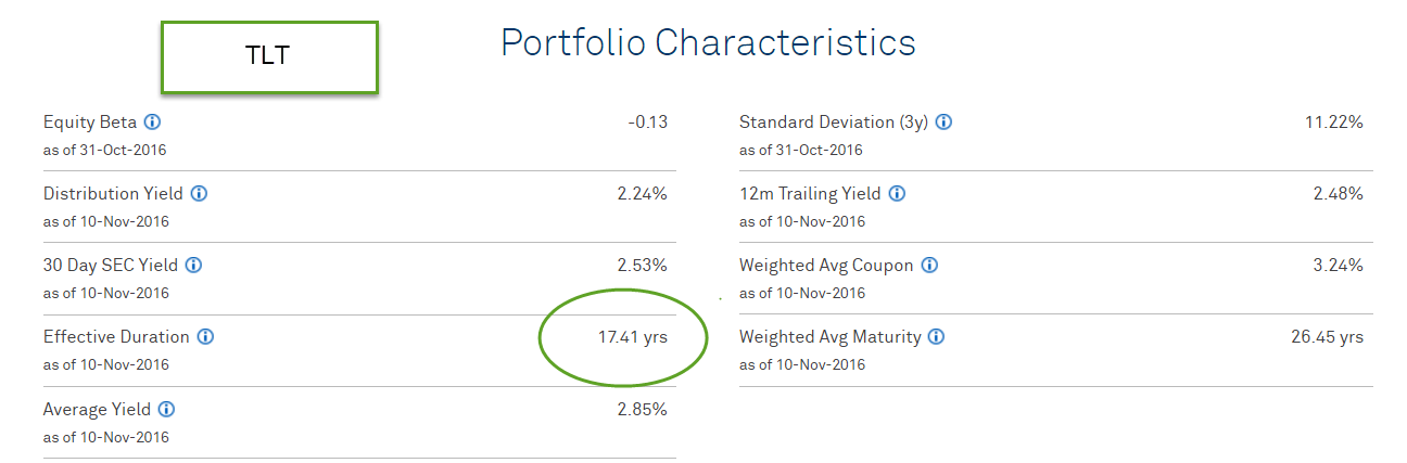
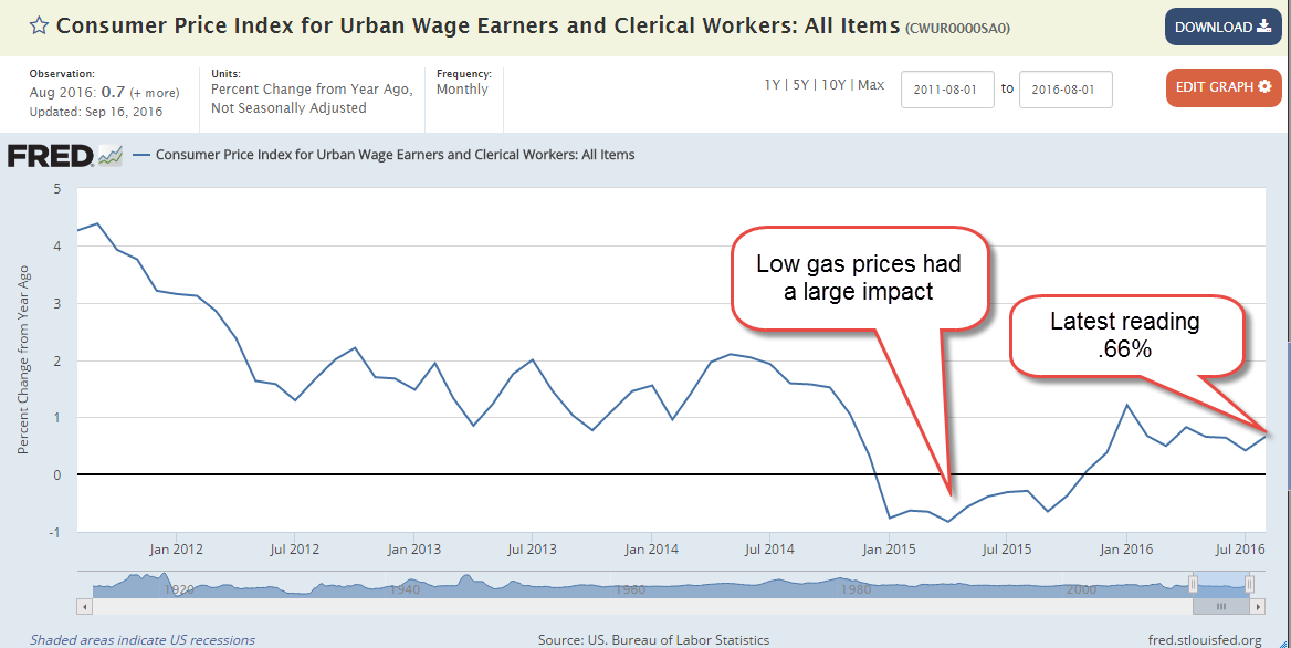
In the weeks since the election, there has been a strong demand for risk, lifting the broad SP500 index by 8%. So how goes it over on the safety side of the ledger? Holders of an index of the total bond market, VBMFX or BND, have seen a price drop of a bit more than 3% since the election, but a net gain of 2-1/4% in the past twelve months.  Almost all of that gain is the yield, or interest earned on the bonds.  Inflation eats up most of that net gain, leaving the bond investor with little net gain for the year, but no loss.

 Morningstar provides a comparison table of various investments.  The AGG broad bond index in their table has an average total return of 2.18% over the past five years.  Yes, this year’s rather low return of 2.25% is better than the five year average.

Vanguard provides a 90 year comparison of various portfolio allocations and it is the first one on the page that I’ll turn to.  Over 90 years, the average total return of interest and price appreciation on a 100% fixed income, i.e. bond, portfolio is 5-1/4%, or 3% more than this year’s total return.

In today’s low yield universe, there is little difference, or spread between today’s yield on a broad bond index and that on a broad stock index.  Over that 90 year period, stocks have averaged 10% per year total return.  The difference between the average total return on bonds and stocks is almost 5% and is called the risk premia.  It means that, on average, a bond investor sacrifices 5% annual return for the income and the relative price stability of bonds. That’s the 90 year average.  The 5 year average tells quite a different story: a 15% per year total return for the SP500 vs 2.18% for a broad bond index.  That risk premia is 2-1/2 times the 90 average.   Seniors and others needing safety have paid a high price.

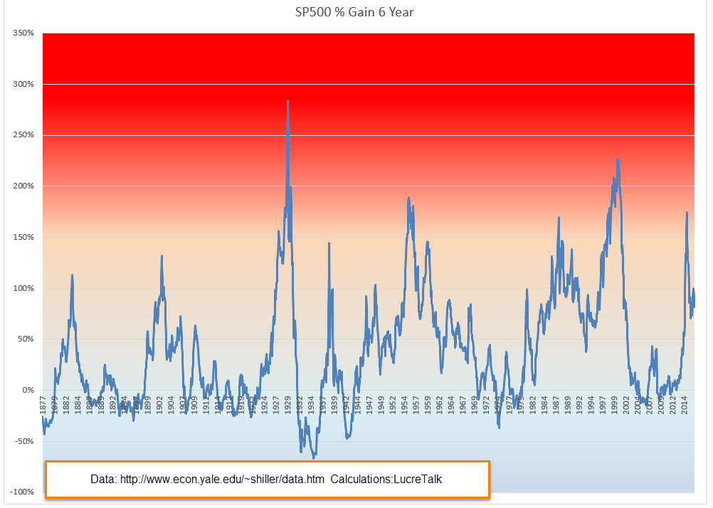
OR…let’s look at this from a different perspective.  In the long run, the law of averages is like gravity. What price would the SP500 be if its total return were more in line with the 90 year average of 10%?  The answer is a price that we last saw during February of this year – about $1840.  That is an 18% drop from today’s current price of $2264.

As the generation of boomers continues to draw down savings to supplement their income, we can expect that price stability will become more valued.  That should balance some of the downside price risk of owning bonds in an environment of rising interest rates.  There are some countervailing forces.  Oil states may derive more than half of their revenue from profits based on the price of oil.  When oil prices were high, the sovereign funds of these states bought U.S. Treasuries and other assets with the excess profits.  As prices declined since mid-2014, the lower revenues have produced budget deficits in those countries dependent on oil.  They have already sold some assets and will continue to do so if prices remain below $60 a barrel.

Comfortability Ratio

The Vanguard table of returns for various allocations (see above) shows that a 60% stocks/ 40% bond portfolio allocation (60/40) produces the best total returns of the choices for a balanced portfolio.  Let’s look at a comfortability ratio – the average return divided by the percent of years with a loss, or %AR / %YL.  This can be an important psychological ratio for those approaching and in retirement.

As many studies have shown, we give more weight to losses than gains.  We are naturally risk averse, and especially so as we near the end of our working years.  Higher comfort ratios are safer.  A 40/60 and 50/50 allocation have comfort ratios of .44.  Their average return is 44% of the percent of years that an investor suffers a loss.

Ranked by this comfort ratio, the surprise is that a 60/40 allocation acts more like a growth, not a balanced, allocation.  70/30 and 80/20 growth allocations have the same .37 comfort ratios as the 60/40.  On a more surprising note, a strongly agressive 90/10 allocation with a .38 ratio  has a better comfort ratio than any of these growth allocations.  Here’s a table:

Allocation Avg % Years Comfort Ratio
                   Return    With Loss
40/60 7.8 17.7 .44
50/50 8.3 18.8 .44
60/40 8.7 23.3 .373
70/30 9.1 24.4 .373
80/20 9.5 25.5 .373
90/10 9.8 25.5 .384
100/0 10.1 27.8 .364

Allocation based on income needs

As an alternative to conventional allocation models using percentages, an investor might keep five years of income needs in bonds and cash and devote the rest to equities. An important caveat: income needs do not include emergency cash. Using this model, an investor who needed $20K from their portfolio each year, would keep $100K in bonds and cash, and put the rest in stocks.  A 35 year old with no income needs would have 100% in equities.  This model naturally becomes more conservative as the portfolio is drawn down.

For two years the stock and bond market have seen little net change.  Investors might have become complacent.  Since the election, the shift in sentiment has been strong and investors should check their year end statements and make adjustments based on their needs and targets.

////////////////////////////

In a country far, far away….

Cue the Star Wars theme. Dah, dummm, dah, dah, dah, dummmmm.  In 2008, China overtook Japan to become the country that holds the largest amount of U.S. Treasuries. Since this summer, China has been selling Treasury bonds to support its currency, the yuan, and is now again in 2nd place.  As long as the dollar continues to rise, China is likely to continue this practice which will maintain a slight downward pressure on bond prices.

Optimism Reigns

Dec. 11, 2016

For the second week since the election the SP500 index rose more than 3%, reversing a slight loss the previous week.  The SP500 has added 160 points, or 7.6%, in total since the election.  Barring some surprise, the market looks like it will end the year with a 10+% annual gain, all of it in the 6 – 7 weeks after the election. Small cap stocks have risen 17% in the past five weeks.  Buoyed by hopes of looser domestic regulations, and that international capital requirements will be relaxed, financial stocks are up a whopping 20% in the same time.

Having held their Senate majority, Republicans now control both branches of Congress and the Presidency but lack a filibuster proof dominance in the Senate.  They are expected to pass many measures in the Senate using a budget reconciliation process that requires only a simple majority. The promise of tax cuts and fewer regulations has led investment giants Goldman Sachs and Morgan Stanley to increase their estimate of next year’s earnings by $8 – $10.  Multiply that increase in profits by 16x and voila!  – the 160 points that the SP500 has risen since the election.  The forward Price Earnings ratio is now 16-17x.

Speculation is about what will happen.   History is about what has happened. The Shiller CAPE10 PE ratio is calculated by pricing the past ten years of earnings in current year’s dollars, then dividing the average of those inflation adjusted earnings into today’s SP500 index.  The current ratio is 26x, a historically optimistic value.  The Federal Reserve is expected to raise interest rates at their December meeting this coming week.

As buyers have rotated from defensive stocks and bonds to growth equities, prices have declined.  A broad bond index ETF, BND, has lost 3% of its value since the election.  A composite of long term Treasury bonds, TLT, has lost 10% in 5 weeks.  For several years advisors have recommended that investors lighten up on longer dated bonds in anticipation of rising interest rates which cause the price of bond funds to decline.  For 6 years fiscal policy remedies have been thwarted by a lack of cooperation between a Democratic President and a Republican House that must answer to a Tea Party coalition that makes up about a third of Republican House members.  The Federal Reserve has had to carry the load with monetary policy alone.  Both former Chairman Bernanke and curent Chairwoman Yellen have expressed their frustration to Congress.  If Congress can enact some policy changes that stimulate the economy, the Federal Reserve will have room to raise interest rates to a more normal range.

//////////////////////////////

Purchasing Manager’s Index

The latest Purchasing Manager’s Index (PMI) was very upbeat, particularly the service sectors, where employment expanded by 5 points, or 10%, in November.  There hasn’t been a large jump like this since July and February of 2015.  For several months, the combined index of the manufacturing and service sector surveys has languished, still growing but at a lackluster level.  For the first time this year, the Constant Weighted Purchasing Index of both surveys has broken above 60, indicating strong expansion.

The surge upward is welcome, especially after October’s survey of small businesses showed a historically high level of uncertainty among business owners.  This coming Tuesday the National Federation of Independent Businesses (NFIB) will release the results of November’s survey.  How much uncertainty was attributable to the coming (at the time of the October survey) election?  Small businesses account for the majority of new hiring in the U.S. so analysts will be watching the November survey for clues to small business owner sentiment.  Unless there is some improvement in small business sentiment in the coming months, employment gains will be under pressure.

////////////////////////////

Productivity

Occasionally productivity growth, or the output per worker, falters and falls negative for a quarter.  Once every ten or twenty years, growth turns negative for two consecutive quarters as it has this year. Let’s look at the causes.  Productivity may fall briefly if businesses hire additional workers in anticipation of future growth.   Or employers may think that weak sales growth is a temporary situtation and keep employees on the payroll.  In either case, there is a mismatch between output and the number of workers.

During the Great Recession productivity growth did NOT turn negative for two quarters because employers quickly shed workers in response to falling sales.  The last time this double negative occurred was in 1994, when employment struggled to recover from a rather weak recession a few years earlier.  For most of 1994, the market remained flat.  In Congressional elections in November of that year, Republicans took control of the House after 40 years of Democratic majorities.  The market began to rise on the hopes of a Congress more friendly to business.  Previous occurrences were in the midst of the two severe recessions of 1974 and 1982.   As I said, these double negatives are infrequent.


////////////////////////////

The Next Crisis?

The economies of the United States and China are so large that each country naturally exports its problems to the rest of the world.  The causes of the 2008 Financial Crisis were many but one cause was the extremely high capital leverage used by U.S. Banks.  A prudent ratio of reserves to loans is 1-8 or about 12% reserves for the amount of outstanding loans.  Large banks that ran into trouble in 2008 had reserve ratios of 1-30, or about 3%.

Now it is China’s turn.  Many Chinese banks have reported far less loans outstanding to avoid capital reserve requirements.  How did they do this?  By calling loans “investment receivables.”  It sounds absurd, doesn’t it?  Like something that kids would do, as though calling something by another name changes the substance of the thing.  70 years ago George Orwell warned us of this “doublespeak,” as he called it.  Reluctant to toughen up banking standards for fear of creating an economic crisis, the Chinese central bank is planning a gradual move to more prudent standards that will take several years.  However, it is a crisis waiting for a spark.  Here’s a Wall St. Journal article on the topic for those who have access.

/////////////////////////

Election Volatility

November 13, 2016

Sometimes the hardest thing an investor can do is nothing.  That’s pretty much what a casual investor with a balanced portfolio should do in response to the election results.  With a portfolio of 57% stocks and 43% bonds and cash, my total portfolio has risen 1/2% this week, or much ado about nothing.  Let’s dig into this week’s election results and the market’s reaction.

Donald Trump, the President-elect, has long maintained that his campaign was a movement and was proved right this past Tuesday.  White voters from rural districts around the country rallied in strong numbers to Trump’s promise to straighten up Washington.

Voters generally want a change of direction after one party has occupied the White House for two terms and this election proved to be no different. In the modern era of politics, only H.W. Bush was able to gain a 3rd Presidential term for the Republican party in 1988 after two terms of Ronald Reagan.  Countering the emotion and momentum of the Trump movement on the right were the voters on the left who passionately turned out for Bernie Sanders in the Democratic primaries.  Voters and superdelegates chose the establisment candidate, Hillary Clinton.  Some say that the process and the rules favored Clinton over Sanders.  His supporters are convinced that Sanders could have beat Trump.  Movement against movement.

In the past decade, voters have expressed a preference for rallying cries, for mantras of momentum like “Si se puede!” (Obama), “Build the wall!” (Trump) and “Medicare for all!” (Sanders).  Candidates must learn to condense their message into a short slogan that can be easily waved.  McCain, Romney and Clinton never found a verbal cadence that would act as a catalyst for voters to enthusiastically join the parade.  Sarah Palin, McCain’s Vice-Presidential candidate in 2008, understood the need for slogans.

 Note to future Presidential candidates who would like to actually win:  criticize the candidate, not that candidate’s supporters.  Hillary Clinton made the same mistake that Romney made in the 2012 election – disparaging their opponent’s voters.

Election night.  As a Trump victory became increasingly probable, global markets began to sell risk (stocks) and buy safety (bonds).  In the early morning hours after the polls closed, the networks called the state of Wisconsin for Donald Trump and put him over the threshold of 270 votes in the Electoral College.  Several  minutes later, about 2:45 AM on Nov. 9th, we learned that Hillary Clinton  had called Donald Trump to concede and wish him luck.  Dow Futures were down about 4% at that point.  Japan’s stock market was down 5.5%.  The yield on the 10 year Treasury note was down 7.22%, meaning that the price was up about 8% as investors in world markets were seeking the safety of U.S. debt.  Emerging markets fell in anticipation of protectionist trade policies under a Trump administration.

About 3 A.M.  President-elect Trump began to give a sedate and rational acceptance speech that began with a gracious nod to Hillary Clinton’s fight.  He spoke of unity, healing and more importantly, infrastructure spending and tax cuts.  With control of the Congress and Presidency in Republican hands, there was real hope that Washington could end the years of stalemate and finally implement fiscal policy to rescue a economy that had been kept afloat by an exhausted monetary policy for six years.

The overseas markets began to turn around.  By the time U.S. markets opened more than six hours later, stocks and Treasuries had reversed.  Stocks were now off less than 1/2% and Treasury prices were down severely.  TLT, a popular ETF for long term Treasuries, opened about 2% lower, a price swing of 10%.  EEM, a composite of Emerging Market stocks, opened up almost 3% down and lost ground during the trading session.  By week’s end the SP500 had risen 3.8% for the week, and EEM had fallen by that same percentage.

This week’s action in the bond market was a good example of the mechanics of bond pricing so let’s look at the price action and what it says about the future guesses of the direction and extent of interest rates.  First, bond prices move inversely to interest rates.   The extent that these prices move is measured by a bond’s duration.  Here is a link to the iShares page for the TLT ETF on long term Treasuries.  I have captured a section of the page with the duration highlighted.

If you have a bond fund, the mutual fund company will state the bond duration as well.  What does this tell you?  Leverage.  Duration tells you the approximate change in price for a 1% change in interest rates.  In this case, a 1% increase in interest rates will generate about a 17% decrease in price.  Because TLT is a composite of long term Treasuries, its price is more sensitive to changes in interest rates, or the consensus on interest rates six months to a year in the future.  The price of TLT fell 7.4% this week as traders repriced future interest rates.  With some grade school math, we can calculate what traders are guessing interest rates will be a half year to a year from now.

The Fed last raised rates at the end of 2015, putting them at approximately 1/4% – 1/2%.  In July, the price of this ETF was about $142.  It closed this week at $122, a decline of 14% from the summer high. Now we divide the 14% by the bond’s duration of 17.41% to get a ratio of .80.  This is the new guess of how much interest rates are likely to rise – approximately 3/4% – 1%.  By the fall of 2017, traders are betting that the benchmark Fed interest rate will be about 1.25% to 1.5%.

Let’s look at a more balanced composite bond ETF that financial advisors might recommend for casual investors.  Vanguard has a more conservative composite ETF whose ticker symbol is BND, with a duration of 5.8, about a third of the TLT ETF. (Spec Sheet here)  This week BND lost almost 2% and is down almost 4% from its summer high.  When we divide 4% by 5.8% (the duration in percentage terms) we get a guess of about a .7% raise in interest rates.  Because BND contains shorter term bonds, this guess is slightly below that of TLT.

Why are traders betting on more aggressive interest rate increases after Donald Trump was elected?  He has spoken about infrastructure spending and tax cuts, two fiscal stimulus programs that will likely spur inflation upward.  With a Republican party that has control of the Presidency and both houses of Congress, these measures are likely to be passed in some form.  Some sectors of the economy will likely benefit from more infrastructure spending so they rose this week.  Shares in technology giants like Apple and Google fell as traders switched money among sectors but are still up by healthy margins since February lows.

Let’s say that next March comes and the Trump White House and the House Budget Committee can not come to terms on either of these programs.  Investors would likely reprice interest rate expectations and lower them, causing the price of bond ETFs or mutual funds to rise.

/////////////////////////////////

Miscellaneous Election Notes

I’ll share a distinction that NPR’s David Folkenflik made this week.  Those on the left took Donald Trump literally, but not seriously.  Those who voted for him took him seriously, but not literally.

During Thursday’s trading the Mexican peso fell to 15.83 per dollar, the lowest since 1993 when Mexico reset their currency. Why the big drop?  Trump has repeatedly said that he would cancel the NAFTA agreement that binds Mexico, Canada and the U.S.  The NAFTA agreeement requires only a 6 month notification before termination.  There is some disagreement whether the White House would need Congressional approval to cancel NAFTA which might delay the action.  Some in the Republican party like free trade agreements and are likely to put up a fight.  Some analysts think that the devaluation of the peso could lead to a recession in Mexico, which was already under economic pressure due to falling oil prices.

131 out of 231 million registered voters cast their vote in this election, slightly below the voter total in the 2008 election. (538)  Trump and Clinton each took 26% of registered voters.

The Trump White House can reverse Obama’s executive action on the Keystone pipeline and re-initiate construction.  It will likely amend or repeal tentative proposals to mitigate climate change.

Why did pre-election polls get it so wrong?  According to Pew Research, more than a third of households would respond to a survey a few decades ago.  Now it is only 9%.  Statisticians must tweak this rather small sample to make it more representative of the population as a whole.  A particular demographic constituent in the sample – say white working class men – might be underrepresented in the survey.  Survey methodology then gives the opinion of relatively few sample respondents more weight than it actually has in the general voter population.

Some statisticians recommend using economic and demographic algorithms to gauge future election results based on actual past voting records.

Of the 700 counties that voted for Obama in 2012, a third of those voted for Trump in 2016.  Polls indicated that Hillary Clinton would capture the majority of the white college-educated vote for the first time in decades but she failed to do so.  More white voters voted for Obama than Hillary.

A third of Democrats in the House come from just three states:  California, New York and Massachusetts.  This concentration may answer to the concerns of those states but indicates that the party has become out of touch with the voters in many states.

Each time a Democratic candidate is elected President, unfounded rumors circulate that the new President will take away people’s guns.  People rush out to buy guns.  Trump’s surprise win caused the stock of gun maker Smith and Wesson to decline 22% in a couple of days.

On the other hand, many women feared that Trump and a Republican Congress would restrict birth control and stocked up in the days after the election. Here is a map of abortion regulations in the states before the 1972 Supreme Court’s decision in Roe v. Wade.  Abortion was more permitted in the southern states than the northeast states.

Here‘s a state-by-state breakdown of the vote from NPR.

Price Plateau

October 30, 2016

Market watchers use several indicators to gauge the valuation of the broader stock market.  The P/E ratio (Price/Earnings), P/D ratio (Price/Dividend) and Shiller CAPE ratio (Cyclically Adusted Price/Earnings) are quite common and I will look at a fourth indicator, the percentage gain in the SP500 index over a six year period.  As we will see, when gains reach a certain height, there are two alternatives that follow:  1) a crash or other steep decline in price, and 2) a flattening of price for approximately 18 months.

Use of any of these indicators – PE, PD, CAPE or this one – would not have helped an investor avoid the 2008 crisis.  Why?  Because they gauge valuation.  The 2008 crisis was a financial crisis based on bad judgment and fraud.  At the time of the crisis, the index had  gained 40% in the past six year period, about the average six year gain over the past 140 years.

Average annual gain – 6%

The average annual gain is a bit under 6%.  The median gain is 29% over a six year period, or a 4.2% annual rate.  Add in the current 2% dividend rate and the median expectation is 6.2% annual gains in the stock market based on the past 140 years. Some public pension funds are still using 7.5% expected annual gains and that will probably be the next crisis in the coming decade.

Five Year Rule

Methodology. Why did I choose a six year period?  Did I run a bunch of simulations to get the most dramatic period?  No.  It’s the first number I picked and the reason I picked it is simple:  it is one year more than the five year rule.  Financial advisors will usually recommend that their clients do NOT keep money in the stock market that they will need in the next five years.  Why? The volatility in the market could cause an investor to sell at precisely the wrong time in order to access funds.  Even at the worst depths of the 2008 crisis, after more than 50% losses, the SP500 index was only 11% less than it had been six years earlier.  This is why advisors use the five year rule.

SP500 Data

Below is a chart of the percent gains in the SP500 index after a 6 year period.  I’ll call the six year gains “6Gain” to save some typing.  The data is courtesy of Robert Shiller who wrote the book “Irrational Exuberance” which first introduced the concept of the Shiller CAPE ratio, an inflation adjusted P/E ratio.

1929 Peak

Let’s look at examples of steep price declines when the percent gains have just gotten too high. The 1929 crash was truly historic.  That’s the highest spike in the chart above.  In November 1928, the 6Gain first crossed above the 150% mark that signals an strong overvaluation.  The market should have started to flounder but lax lending rules probably helped fuel further price gains.  Many people with acceptable credit could borrow money against stocks and many did, chasing the strong upward trend in the market.  Over the next ten months the market climbed another 20%.  The decline began in mid-September 1929 (Dow chart) but was seen as a well deserved correction to the summer exuberance. At the end of September 1929, the market had gained 284% in six years, the highest 6Gain on record and a percentage gain that may go unbroken.

…and Crash

In October 1929 the market continued to lose ground, forcing the sale of borrowed securities to meet margin calls.  Margin selling contributed to the downward momentum but the sustained selling woke investors up to the fact that the market had climbed too far and too fast.  The selling culminated in a gut wrenching 23% loss on Black Tuesday, October 29th (Account of crash – I disagree with the author on valuation).

Seeking Average

It took 18 months for the market to correct to a 6Gain that was average (39% over 140 years). By that time in May 1931, the market had lost 55% of its value.  From 1931 to 1936 any money invested in the stock market six years earlier had shrunk. In 1934, six year LOSSES, not gains, approached 60%. My parents grew up during the Depression and were taught that the stock market was a reckless gamble made only by rich people who could afford to lose some of their savings.

Black Monday

These overvaluation crashes are rare, thank God.  The next one came more than 50 years later, on “Black Monday” in  October 1987, when the index lost 20% in ONE DAY, almost as much as Black Tuesday in 1929.  At that time, the 6Gain was 169%.  I can still remember where I was when that one went down. Traders could not get some of their orders filled and that began a panic in the market. Some radio pundits warned of another depression.  I had no savings in the market but I was worried that my relatively new business would go belly-up. Most of the 24% lost in two months was done in that one day.  It took a whopping six years for the 6Gain to fall to average.

The Plateau

Those are the only two examples of severe price crashes because of overvaluation.  The more common result of overvaulation is a plateau, a flattening of prices for about 18 months, followed by by a fork – up or down.  The price plateau simply tells us that a fork in the road is coming.  The over-valuation tells us to expect a price plateau.

The dot-com boom

Let’s look at the dot-com boom in the late ’90s. At the end of 1994, the SP500 index closed at 460.  Less than six years later, in the fall of 2000, the index crossed above 1500, more than triple the price in that short six year period. The 6Gain peaked at 227%. At mid-1999 the SP500 started to stall out above 1350.  Promises of huge profits to be made by internet companies were beginning to evaporate as those companies burned through cash at an alarming rate in their effort to capture a segment of the market. It would take another year before the market peaked near 1500.  By the end of 2000, eighteen months on this rounded plateau, prices were about 1350 again.  For almost two years they declined till the index had lost more than 40% of its value.  Coincidentally, this low was reached when the 6Gain finally dropped to the 140 year median of 29%.

The Fabulous Fifties

Let’s look at some older and milder examples to develop some context. In mid-1955, the index had gained almost 190% in six years. It continued to climb for another 6 – 8 months before falling back.  In the spring of 1957, the index stood at the same level as it had eighteen months earlier.

In mid-1959 the index had gained almost 150% in six years.  The index lost 10% over the next 6 months but by early 1961, about 18 months later, the index had gained back its lost ground.

In mid-1938, we see the same price plateau after a six year gain of 150%.

Recent

As we can see on the chart, these 6Gain spikes are infrequent.  Now let’s look at the most recent spike in the 6Gain – March 2015.  The SP500 index was near where it is today.  In fact, this may be the flattest price plateau in history.  The stock market was overvalued but with bond yields so low, where was an investor to go?  Real estate, commodities, gold and other alternative investments have gone up and down the past 18 months as traders tried to take advantage of mis-matches between expectations and reality.  The trend for the average investor?  No trend.

During this 18 month plateau, the 6Gain has fallen to 82% – a good sign – but still twice the average 6Gain.   Wouldn’t it be nice if there was a law that the 6Gain must fall to the average before the stock market takes on a definite trend in either direction?  No such law.  What we do see with ironclad regularity is a price plateau when the 6Gain crosses above 150% and that the plateau lasts about 18 months.  It has been 18 months and we should be nearing the edge of that plateau.

Closing Thoughts

As October draws to a close, we may have three months in a row where the month ending price (Close) is less than the price at the beginning of the month (Open).  Normally, 3 down months in a row would be a sign of more pain to come but the differences each month have been negligible and could be pre-election hesitation.  There is enough to be hesitant about.  The Shiller CAPE ratio is about 26, 10 points above the median of 16.  Due to declining oil prices, profits in the SP500 aggregate of companies have fallen for five quarters in a row and…

The Election

Trump has been losing ground in recent polls, enough so that the Senate seems more likely to turn Democratic.  This Senate cycle favors Democrats who have fewer seats up for re-election than Republicans.  In 2018, the cycle will favor Republicans.  As the gap in the polls widens, some begin to fear that a rout in the Presidential race could cascade into the House where Republicans hold what seemed to be an impregnable lead of 60 seats (Wikipedia article).  If the Democrats should take the House, they will control the Presidency, Senate and House.  Tax increases on those with upper incomes would be a certainty for 2017, as Hillary has promised.  This could cause a rush of selling in 2016 to avoid higher capital gains tax rates.  An unlikely but not impossible scenario may be contributing to the hesitation.

Portfolio Mix

October 23, 2016

About 30 years ago, after a series of social security and income tax increases in the early ’80s, I had a spirited discussion with my dad about what I thought was a transfer of money from my generation to his.  Extremely low interest rates for the past eight years have reversed that process.  Millions of older Americans who have saved throughout their working years are getting paid almost nothing on that part of their savings held in safe accounts.  Older Americans take less risk with their savings and it is precisely these safer investments that have suffered under the ZIRP, or Zero Interest Rate Policy, of the Federal Reserve.  That money is implicitly transferred to younger generations who pay less interest for their auto loans, for their mortgages, for funds to start a business.

The chairwoman of the Fed, Janet Yellen, is at the leading edge of the Boomer generation born just after WW2.  No doubt she and other members of the FOMC are well aware of the difficulties ZIRP  has had on other members of her generation. Because the Boomers have been a third of the population as they grew up, they had a consequential effect on the country’s economy and culture.  Their income taxes have funded the socialist policies of the Great Society.  They have funded the recovery from the Great Recession.  Ten years from now politicians will regretfully announce that, in order to save Social Security, they must means test Social Security benefits to reduce payments to retirees with greater assets.  Once again, politicians will tap the Boomers for money to fund the policy mistakes that politicians have made for the past few decades.

//////////////////////////

Portfolio Mix

Each year Warren Buffett writes a letter to shareholders of Berkshire Hathaway, the holding company led by Buffett.  His 2013 letter made news when Buffett recommended that, after this death, his wife should invest their personal savings in a simple manner: 90% in a low-cost SP500 fund, and 10% in a short term bond fund, an aggressive mix usually thought more appropriate for younger investors.  Earlier this year, a reader of CNN Money asked if that would be a practical idea for an older investor approaching or in retirement.

After running several Monte Carlo simulations, the advice was NO, but the reason here is interesting.  The 90-10 mix does quite well but has a lot of volatility, more than many older investors can stomach.  An investor in their late 40s or early 50s who is making some good money might relish a market downturn.  Could be twenty years to retirement so buy, buy, buy while stocks are on sale.  If they go down more, buy more.

The sentiment might be entirely different if the investor is ten years older.  Preservation of principle becomes more of a concern.  Why is this?  Let’s look at a sixty year old woman who plans on working till she is seventy so that she can collect a much bigger Social Security (SS) check.  During her retirement years she will have to sell some of the equities she has in a retirement fund or taxable account to supplement her SS check.  However, the majority of those sales won’t take place for 15 – 20 years.  Why then is she more concerned about a market downturn than she might have been at 50 years old?  Do we simply feel more fragile at 60 than we do at 50?  I suppose it’s different for each person but, in the aggregate, older investors are more cautious even if the probability math says they don’t have to be as careful.

With two weeks to go before the election, the stock market has lost some of its spring/summer fire.  Looking back 18 months, the market has had little direction and is now about the same price it was in January 2015.  Companies in the SP500 have reported five consecutive quarters of losses, and the analytics firm Fact Set estimates that there will be a small loss in this third quarter of the year, making six losses.  Energy companies have been responsible for the bulk of these losses, so there has not been a strong reaction to the losses in the index as a whole.

BND, a Vanguard ETF that tracks a broad composite of bonds, is just slightly below a summer peak that mimicked peaks set in the summer of 2012 and again in January 2015.  However, this composite has traded within a small percentage range for the past two years.  In fact, the same price peaks near $84 were reached in 2011 and 2012.  Once the price hits that point, buyers lose some of their enthusiasm and the price begins to decline.  Most of us may think that bonds are rather safe, a steadying factor in our portfolio.  Few people are alive that remember the last bear market in bonds because this current bull market is about thirty years old.

Oil has been gaining strength this year.  An ETF of long-dated oil contracts, USL, is up about 15% this year.  Because it has a longer time frame, it mitigates the effects of contango, a situation where the future price of a commodity like oil is less than the current price.  As the ETF rolls over the monthly contracts, there is a steady drip-drip-drip loss of money. Short term ETFs like USO suffer from this problem.  Of course, long term bets on the direction of oil prices have been big losers.  In 2009, USL sold for about $85.  Today it sells at about $20. Here is a monthly chart from FINVIZ, a site with an abundance of fundamental information on stocks, as well as charting and screening tools. The site gives away a lot of information for free and there is a premium version for those who want it.

These periods of low volatility may entice investors into taking more chances than they are comfortable with so each of us should re-assess our tolerance for volatility.  In early 2015 there was a 10% correction in the market over two months.  How did we feel then?  The last big drop was almost 20% in the summer of 2011, more than five years ago.  The really big one was more than eight years ago and memories of those times may have dimmed.  If you do have easy access to some of your old statements, a quick look might be enough to remind you of those bad old days when it seemed like years of savings just melted away from one monthly statement to the next.

Yes, we are due for a correction but we can never be really sure what will trigger it and these things don’t run on schedule.  On a final, dark note – price corrections are like our next illness. We know it’s coming.  We just don’t know when.

Pool and Flow

October 2, 2016

A few weeks ago, I introduced two concepts: stock and flow. I’ll develop that a bit to help the reader analyze their portfolio with a bit more clarity.  To avoid confusion between stocks, as a type of investment, and the concept of a stock as in a reservoir or pool of something, I’ll refer to the concept as a pool and stocks as a type of investment.

Leverage

Each month we might check our investment and bank statements to find that the value has gone up or down.  In any one day only a tiny portion of stocks and bonds trade, yet these transactions determine the value of all the unsold assets, including the ones on our statement.  As I mentioned a few weeks ago, the flow from a reservoir of water determines the value of all the water in the reservoir.  It is like the butterfly effect, the idea that the fluttering of a butterfly’s wings in Mexico can cause a typhoon in southeast Asia.  In financial terms, when a small event has a large influence it is called leverage. A flow, a transaction, is the  catalyst for a transfer of value from one asset to another.

Let’s look at an example.  We buy a 1000 shares of the XYZ biotech firm for $10 a share, for a total investment of $10,000.  The next day the FDA announces that, contrary to expectations, they will allow a drug trial to proceed to Phase 3.  XYZ’s stock price rises 10% in response to the news.  The market price of our investment is now worth $11,000.  Where did the other $1000 come from?

Transfer of Value 

An asset value rose, so the value of another asset pool fell as the value is transferred from one asset to pool to another. Yesterday $10,000 of cash was worth 1000 shares of XYZ.  Today, that $10,000 of cash is worth only 909 shares of XYZ.  This is a different way of looking at cash – not as a liquid medium with  a stable value – but as an asset with an erratic value.

Cash = Investment 

What is cash?  It is an investment of faith in the United States.  We might give it a stock symbol like CASH and I’ll use that stock symbol to distinguish cash when it acts as an asset.  Stockcharts.com allows users to track the relationship between two stocks, or to price one stock in terms of another. We do by typing in the a stock symbol ‘A’ followed by a colon and a second stock symbol ‘B’.  Stockcharts will then show us the value of A priced in B units.  Below is the chart of Google (GOOG) priced in Apple (AAPL) units, or GOOG:AAPL.

On the left side of the chart in early 2014, Google’s stock was worth about 6.25 “Apples.”  By mid-2015, Google’s stock had fallen to 4.25 Apples.  Did Google’s value fall or Apple’s value rise?  Let’s imagine that we live in a world without money, as though we had taken the red pill as in the movie “The Matrix.”  Without a fairly constant measure like cash, we simply don’t know the answer to that question.  Imagine that each investor gets to choose which asset they want their monthly statement priced in and that our choice is Apple.  Over a year and a half, we see that we have lost about a third of the value of our portfolio of Google (6.25 / 4.25 = about 2/3).  We can’t stand the continuing losses anymore and sell our Google stock and get 4.25 units of Apple. It is now September 2016 and we still have 4.25 units of Apple because Apple is our measure of value.  Had we continued to hold the Google stock, we would have 7.29 Apple units.

What is CASH worth?

Now let’s turn to a slightly different example.  We are going to price CASH in Apple units, the inverse or reciprocal of how we normally do things.  When we say that Apple’s stock is $100, for example, we are pricing Apple stock in CASH units, or AAPL:CASH.  Instead we are going to look at the inverse of that relationship: pricing CASH in Apple units.  Remember, we are no longer in the matrix.

We begin with the same portfolio, 6.25 Apple units in early 2014.  We think that this CASH asset is going to do better than Apple, so we sell our Apple units for CASH and get 68 cash units for each Apple unit, a total of 425 cash units.  In mid-2015, we find that our CASH units are now worth only 3.5 Apple units.  We have lost about 45% in a year and a half!  We sell our CASH units and get 3.5 Apple units which is what we still have in this latest statement 15 months later.

Our losses are even worse than that.  Each year, Apple gives the owners of its shares another 2/100ths of a share as a dividend.  The owners of CASH get only 1/100th of a cash share each year.  Apple pays those dividends from its profits.  For owners of CASH, a financial institution pays the dividends from its profits. While the Federal Reserve, a creation of the Federal Government, doesn’t directly “set” interest rates it effectively does so through the purchase of bank securities.  Each dollar bill is equivalent to a share in an entity called the United States and it is ultimately the U.S. government that largely determines the dividend rate that is paid on safe investments like savings accounts.

Stock dividends compete with cash dividends

To remain competitive with safe investments, Apple only has to pay a little more than the very low dividend rate that savings accounts are currently paying.  If interest rates were 5% instead of the current 1%, Apple would have to devote more of its profits to dividends to appeal to income oriented investors.  By keeping interest rates low, the Federal government effectively allows Apple to retain more of its profits.  Where does Apple keep that extra money?  Overseas and out of the reach of the IRS.  That’s only part of the irony.  If Apple had to pay more of its dividends to the share owners, the share owners would pay taxes on the income. So the U.S. government loses twice by keeping rates low (See footnote at end of blog).

So CASH is effectively owning the stock of an entity called the United States, which doesn’t make a profit.  In the long run, owning the stocks of companies that do make a profit generates much more return to the owner.  Let’s look again at the leverage aspect of stocks and cash.  Earlier I noted the huge leverage involved in stock and other non-CASH asset transactions.  A tiny number of transactions affects the value of a large pool of assets.  On the other hand, millions of CASH transactions take place each day and have little effect on the nominal value of CASH.  So we price highly leveraged assets – stocks, bonds, etc. – in terms of an unleveraged asset – cash.

The functions of cash  

Cash plays several roles. First, as a medium of exchange, it acts as a measuring stick of economic flow in a society. This first role has a symbol – $.  Secondly, as an asset pool, CASH acts as a holding pond, a reserve in the waiting, the first in the asset reservoir to be tapped. Lastly, it acts as an insurance on the principal of other assets, like stocks and bonds.  Let’s call that INS.

Insurance

As an insurance, let’s consider a portfolio of $900 in stocks, $100 INS.  A 10% fall in stocks is reduced to a 9% fall because of the INS position.  Let’s consider the exact same portfolio, except that the investor’s intention is that the $100 is a CASH investment, a reservoir of asset buying power.  The same 10% fall in stocks is now a trigger for additional purchases.  In the first case the $100 is an anxiety reduction fee; in the second, a prediction of a market correction.

An investor might blur the distinction between the functions. Retired people who want to preserve the nominal value of their savings may tend to keep the majority of their nest egg in cash without distinguishing the different functions.  Cash = safety and liquidity. Because cash is used as a yardstick, its nominal value is kept constant.  But what that cash can buy, its purchasing power, changes.  When they need some of that CASH ten years from now, the purchasing power of that asset may have fallen by 30% but the nominal value is the same as it was ten years earlier.

Cash Analysis

As noted before, companies must make a profit or go out of business. Not so the U.S. government. Over time, the rate of a company’s profit growth must exceed the inflation rate, so that stocks give the best investment return in the long run.  Investors would benefit by separating their cash position into its functions, $ and CASH and INS, to understand more clearly what their intentions and needs are for the coming year.  This can be as simple as a piece of paper that we review each year.

Analysis Example 

An example – Cash needs:
1) income for the next year including emergency fund – $50K – $ function.
2) stock market seems awfully high and it has been a while since there has been a 10% correction – $100K CASH function.
3) $30K INS function to help me sleep at night in case there is more than a 10% correction.
Total: $180K.

Why write it down?  Believe it or not, we forget things.

////////////////////////

As a footnote:

Offsetting the tax losses to the government is the fact that some of Apple’s cash consists of cash-like equivalents like Treasury bonds which pay a very low dividend.  Apple loses income because of the low dividend and the U.S. government gains by being able to borrow money from Apple at low rates.

The Fed Feints

September 18, 2016

This week I’ll cover several topics, most of them concerning personal finances.

Social Security and COLA

 Sometime in mid-October the Social Security Administration (SSA) will announce the cost-of-living adjustment (COLA) for social security benefits in 2017 and it will probably be less than 1% (History of previous COLA adjustments).  The COLA is based on the year-over-year increase in the Consumer Price Index (CPI).  In 1982, Congress specified that the SSA use the CPI version for urban workers, called CPI-W. (Info from SSA).  Each month the BLS releases their estimate of inflation, and this week they published their calculation for August – a yearly increase of just .66%.  September’s inflation number may be slightly different but the reality for the average SS recipient is a monthly increase of less than $10 in the average benefit of $1340.

Gas prices fall

For years senior advocacy groups like AARP have argued that a different CPI measure should be used to calculate the COLA.  The alternative measure, the CPI-E, puts more weight on health care expenses and less weight on gasoline and transportation costs because seniors don’t drive as much. So far, Congress has not adopted any changes to the methodology of calculating inflation for retirees.

In late 2014 gasoline prices began to fall and this had a significant impact on measured inflation in 2015, as we can see in the chart below. Although gas prices remain low, they have stabilized so that they will have less of an impact on yearly inflation growth in the future.

Reaching For Yield

Investors who are reliant on the income from their investments, including giant pension and endowment funds, typically desire fairly safe investments that will give them a decent return while preserving their principle.  These include high grade corporate bonds (Johnson and Johnson, for example), Treasury bonds, CDs and savings accounts. Abnormally low interest rates have made those traditional investment choices less desirable.

Like a stream diverted, investors have wandered to riskier assets, bidding up the prices of stocks which are considered more likely to retain their value because they pay dividends.

Dividend ETFs 

 As one example, Vanguard’s VIG is a Dividend Appeciation ETF containing of stocks that  have a consistent record of dividend growth of almost 5% per year.  The growth rate is 5%, not the dividend yield. The companies in this basket are household names: Johnson and Johnson, Microsoft, Pepsi, McDonald’s, and Walgreens, to name a few.  Vanguard has an added benefit: a very low expense ratio.  At the end of August, the Price-Earnings (P/E) ratio on this basket of stocks was 24.5 (see here). In the first two weeks of September, the prospect of an interest rate hike in the next few months has put a small dent in the price, and lowered the PE ratio slightly.  Clearly, investors are willing to pay extra for income, and extra for reliability.  The yield on this basket of reliability is 2.1%, just .4% more than a 10 year Treasury.

DVY

iShares’ DVY is a popular dividend ETF that has a less selective basket of stocks.  This basket also includes oil and energy companies that have a 5 year record of paying dividends but may not have a consistent record of dividend growth because of declining oil prices.  Because the criteria is less restrictive, this ETF is cheaper – it has a higher yield of 3.2% and a lower PE ratio of 20.8.

The Fed

After eight years of near zero interest rates, the Federal Reserve has put itself in a corner. Whatever actions or adjustments it takes must be in small increments to avoid causing a sudden repricing of the very asset prices it has helped lift by maintaining a low interest rate environment.

The financial crisis was so severe that the Fed thought it must lower rates to near zero, which choked income flows from savings.  Such a policy could be justified as an emergency measure. The economy had suffered the equivalent of a heart attack and the Fed need to shock it alive.  However, the recovery that followed was so weak that the Fed thought it must continue to keep rates low.  After eight years of ZIRP (Zero Interest Rate Policy), the Fed finds that it has effectively been picking winners and losers. Debtors win, savers lose. The Fed was forced into the role by the inability of a bitterly divided and ineffective Congress to pass fiscal policy solutions.

To fully grasp the effects of Fed policy, let’s take a trip up into the mountains.  Imagine a high mountain lake reservoir with a dam at one end to contain the water.  On the mountains surrounding the lake falls snow and rain that drains into the reservoir.  The dam is opened enough so that it releases a measured stream of water for users downstream.  The lake is a stock. The release of water is a flow.

Now let’s say that there is a drought for a year or two.  The water level in the reservoir begins to fall.  The dam operators reduce the amount of water released and this has a negative impact on downstream farms and businesses who depend on the water. The price for water rises as farms and businesses bid to get more water, a simple case of supply and demand. Land, another store of value, decreases in value because the lack of adequate water has made the land less productive. Assuming the same demand, prices for produce from the land rises.  This is the flow from the land, So the flow from the land rises while the stock value of the land falls.  Water is a different kind of asset, a consumable.  In the case of water, both the flow and the stock value rise during a drought.

Eventually the rainfall increases and the reservoir refills with water.  Now the dam operators release more water and the price per unit of water naturally declines. Now the stock value and the flow value of the water have declined. A greater supply of produce leads to price declines in the flow of produce from the land, while the price of the land itself, the store of land’s value, increases in anticipation of more productivity from the land.

After the crisis is over, flows from both types of assets declines.  The extra stock value of the water is transferred back to the land. The flow of water from the reservoir has been the catalyst for this transfer of value.

Let’s take this simplified situation and use it as an analogy to understand the Fed.  When the Fed adjusts interest rates, it transfers a store of value from one asset class to another. (It involves a number of asset classes.  I’ll keep it simple.) That’s the transfer of stock value.  But there is also a raising or lowering of the price of the flows from each of those assets.

Now let’s imagine that the Fed raises interest rates by 1%, effectively opening up the dam’s sluice gates a little more.  The flow of income shifts from debtors, who must pay more for borrowed money, to savers, who receive more for their savings.  Debt is a store of value and this is where the transfer of value happens.  New debt competes with old debt and lowers the price of existing debt, both corporate and government, so that old debt can generate the same income flows as new debt. Assets like bonds, which generate income flows at lower interest rates are now worth less.  Why buy a safe bond paying 2% when I can buy a safe bond paying 3%?  Dividend paying stocks are worth less unless they can realistically increase their dividend to compete with higher interest rate expectations. Buyers and sellers of these instruments adjust the prices to reflect the new expectations.

The change in flows acts as a catalyst for the transfer of the stock values between assets.  When we are younger and working, we don’t pay much attention to income flows from our savings.  We look at our portfolio statements, check our 401K or savings balances to see how much of a stock of assets we have built up.  We measure these assets in dollars, not value and may come to think that dollars and value are the same.  Income flows are measured in dollars.  The stock those flows come from are measured in value.  In the future, I hope to explore the ways that we try to convert value to dollars.

It’s Never Happened Before

July 24, 2016

It’s often been said that everyone is entitled to their own opinion but not to their own facts.  Repeated experiments have shown that, through a process of cognitive filtering, we do form our own set of facts. First we filter what we recognize, then we assign different degrees of importance to what we do recognize.  The world is a big lump of Play-Doh that we pull parts from then shape it into a personal ball that we call reality.

Several decades ago when computer development and design was still fairly primitive, computer scientists envisioned the develpment of algorithms that allowed computers to act with the mental versatility of human beings. Many hoped that this new technology, called artifical intelligence, or simply AI, would be implanted in robots which would handle menial or dangerous tasks, making our lives both safer and less tedious.  Soon robots were deployed on factory floors and were highly effective at repetitive tasks.  The deployment of AI was but a few years distant, it seemed.

The AI project soon ran into difficulties when robots tried to navigate a room with only a few obstacles.  What was a routine task for a two year old toddler was extremely difficult for a robot.  Programmers struggled to write algorithms to distinguish and describe just the shadows of objects, and were especially frustrated that a puppy a few weeks out of the womb could do a better job at navigating a room than the most beautifully complex algorithm they could devise.

A decade or so later, Google and other tech firms are test driving cars with autonomous navigation.  How have AI algorithms progressed from negotiating the obstacles in a room to navigating a highway at 65 MPH?  Working with behavioral scientists and psychologists, programmers began to uncover a rather unflattering but powerful model of human learning, one that philosopher David Hume had posited almost three hundred years ago.

Hume was just a teenager when Isaac Newton, perhaps the greatest scientist that ever lived, died in 1726.  Newton formulated the fundamental laws of motion and gravitation.  Hume, on the other hand, put forth the radical notion that we can not know cause and effect, only the correlation of events. We can imagine that Newton rolled over in his grave a few times at this proposal. Hume contended the forces of motion that Newton had proposed were highly probable correlations only.

Scientists dismissed Hume’s skepticism.  For all practical purposes, the universe was bounded by the laws of classical mechanics that Newton had devised.  Scientists went on to develop a model of a clockwork universe created by God that obeyed a set of rules invented by God and thank you very much.  There was apparently little more to discover until two scientists, Albert Michelson and Edward Morley, went to measure the aether, a fundamental component of the clockwork universe.  They couldn’t measure it.  This “undiscovery” rocked the world of physics because it undermined the theories of planetary motion, of gravitation, and the behavior of light.  Undiscoveries are as important as discoveries.  A hundred years before the Michelson-Morley experiment, chemists were unable to find phlogiston, the supposed fundamental cause of combustion, and caused a radical revision of chemical theory.

Twenty years after the Michelson-Morley experiment, Albert Einstein presented his Special Theory of Relativity but even that theory could not fully explain gravity.  A decade later and a hundred years ago, Einstein theorized that our perception of falling was an illusion based on our perspective, a vantage point as we were falling along the surface, or field, of space time.  The system of relative motion that he introduced has radically altered the science of physics since.  Einstein had introduced the same skepticism to the physical sciences that Hume had introduced to philosophical inquiry.

During the past two hundred years mathematicians have developed a number of statistical tools to measure not only the correlation between events, but the correlation of our past predictions based on correlation. As processors became more powerful and memory storage more compact, programmers turned to those statistical tools to enrich their AI algorithms. A baby can not find its own hands at first.  Through trial and error the baby develops a sensory system called proprioception that is not confused by the conflicting data from the baby’s eyes.  When the baby moves both hands in opposite directions to the center of her vision, the hands have more of a chance of colliding together.  The sense of touch confirms the contact of the two hands.  There may be a slight sound. The brain learns the coincidence, the correlation of these phenomena and forms a learning model of cause and effect.

Shortly after the financial crisis in 2008, the former head of the Federal Reserve, Alan Greenspan, testified before Congress about his personal set of beliefs of cause and effect in finance. Because this set of circumstances had not happened before, Mr. Greenspan thought that it could not happen.  Didn’t he see the dangers of 30-1 leverage ratios by major banks in the U.S.?, Greenspan was asked.  Yes, he saw them but did not fully appeciate the degree of danger.  The rash stupidity of bank officers, the disregard for their own welfare, surprised and disturbed him most.  He could not understand that intelligent people could act with such utter disregard for their own self-interest.  Of course, the bankers didn’t have to look our for themselves.  They paid politicians in Washington to do that for them.

Greenspan is a very smart man, as are most of the economists and financial wizards who did not understand the dangers of the synthethic debt instruments that were being created and traded.  Why?  Because it had not happened before.  We are all subject to this fault in judgment.  We are so guided by past experience that it skews our judgment, our ability to assess both risk and opportunity.

 It has been seven years since the market low in March 2009, seven years since the official end of the recession that began in December 2007 and ended in June 2009.  The Shiller price earnings ratio of the SP500 index is very much higher than average.  Even the conventional P/E ratio, the TTM or Trailing Twelve Months ratio, is about 23; the historical average is less than 17. Here is an excellent recent review of P/E ratios.  Low oil prices have helped cripple earnings growth for the SP500 index as a whole but even when excluding energy stocks, both revenue and earnings growth has shrunk.  Yardeni Research has put together several graphs to illustrate the trend.

The Money Flow Index (MFI) is an oscillating measure of buying and selling pressures based on both volume and price.  This index usually ranges from 20 to 80 on a scale of 0 to 100.  This month, the 12 month reading of the SP500 fell below 40.  Such a low reading has been associated with a long period of a rather flat market as happened in 1994-1995.  More often, a low reading is associated with subsequent falls in equity prices, as in early 2000 and late 2007.  Toward the end of 2008, this index fell below 20, indicating extreme selling pressure.  We only have past correlations to guide us.

Bond prices are high.  Vanguard’s ETF of intermediate term bonds, those with maturities of five to ten years, are now yielding less than 2%.  As bond and stock valuations have climbed, have we adjusted our portfolio allocation to stay within our guidelines?  Oops, did we kind of forget to even look anymore?  Did we get lulled into a sense of security?

Saving money is a gamble on the fact that we will get older.  Most of us will experience some reduction in our physical abilities, and a corresponding decrease in the amount of income we earn from our labor.  Saving money therefore seems like a really safe bet.  Once the money is saved, though, another series of gambles begins and these bets are far less certain.  Where to put those savings so that we can get a reasonable balance of return and risk?

 For a short time both the stock and bond markets can experience a surge in selling as they did in 2008. When investors are scared, they run like deer into the safety of cash. After the initial reaction, one or the other of these asset groups will continue to feel selling pressure.  This is why most advisors recommend some balance of stocks and bonds. If the stock market were to drop 50%, or the bond market drop 20%, and stay down for five years, would we be able to meet our income needs?  Such a downturn might be welcome to a 35 year old who can buy equities at a lower price.  For seniors near or in retirement who might have planned to convert some of those higher valuations into income, such a downturn can be devastating.  If such a scenario would be a crisis for you, then it is time to assess your situation and perhaps make changes.

Brexit

June 26, 2016

“Should I Stay Or Should I Go?” was a 1982 song by the Clash.  For months, Brits have debated the question of whether to stay in the European Union (EU) ahead of a referendum vote held just this past week and nicknamed “Brexit,” a mashup of British Exit.  Germany and Britain are the two strongest members of the EU and the loss of either from the union would weaken it’s political and economic ties. In the U.K., the campaigns turned vicious and sparked the murder of an MP (story) earlier this month.  In the British Parliamentary system, an MP is similar to a Congressperson in the U.S. House.

In recent polling the advocates of separation, or Leave, appeared to be gaining momentum so that the outcome of the referendum vote seemed deadlocked at 50-50.  A poll in the last days before Thursday’s vote reassured many that cooler heads would prevail and Britain would remain with the EU. Leaders from both the right and left belonged to this coalition, appropriately named “Remain.”

At about 3-4 AM London time, 11 PM New York City time on Thrusday night, a third of the vote had been counted and it was eerily close, with the Leave group having a teensy-weensy lead.  Then half of the vote was counted and the Leavers were up 1% over the Remainers.  As the vote tally continued, it became apparent that – surprise, surprise – the Remainers had won the vote.

Asian markets were active at that time and responded with a severe sell off of risky assets like stocks and rushed into the safe haven of bonds, cash and gold.  Stocks were down as much as 12% initially on some Asian exchanges.  Gold shot up 6%. Neither the U.S. or European markets were open but the Futures markets in the U.S. sank 6% and European futures plunged 9%.

While most Americans were sleeping European markets opened about 8- 9% down. Market makers in Italy could not establish an opening price for a number of Italian bank stocks, which had already been under pressure in recent weeks.  When they did, these stocks had lost a third of their value.  Everyone was selling, few were buying.

The referendum vote still needs to be codified into law before the Brits formally notify the EU that the country is leaving. After that negotiations begin over the trade and diplomatic terms of exit, a process that could take two years.  A rational person might wonder why the panicked selling?  The worry is that this vote may provoke similar votes in other EU countries, which might lead to the eventual dissolution of the EU.  When in doubt, get out.  Traders did.

Earlier this month the WSJ reported that legendary (and semi-retired) investor and billionaire George Soros had returned to his trading desk to make a series of bearish bets on global markets in anticipation of both political and economic turmoil.  Soros became a household name when he made a $1 billion on a bet against the British pound in 1992.  In several hours Thursday night/Friday morning, the British pound lost 10% of its value.  Was this also another killing for Soros?  Soros thinks the break-up of the EU is inevitable (Story)

What should the long term investor do?  January’s dip of 5% was a good time to make an IRA investment.  This may be an equally good opportunity.

Timing Models

May 22, 2016

Long term moving averages can confirm the shifting trends of market sentiment and market watchers customarily watch for crossings of two averages.  The 50 week (1 year) average of the SP500 index just crossed below the 100 week (2 year) average, indicating a  broad and sustained lack of confidence.  Falling oil prices since mid-2014 have led to severe earnings declines at some of the large oil companies in the SP500.  The index is selling for about the same price as the two year average.

What to do?  These crossings or junctions can mark a period of some good buying opportunities – unless they’re not – and that’s the rub with indicators like this one.  Downward crossings typically occur after there has already been a 5 – 15% decline from a recent high.  If an investor sells some stocks at that time, they wind up selling at an interim low, and regret  their action when the market rises shortly thereafter.  They should have bought instead of sold.  AAAARGHHH, a false positive!  Twice in the 1980s, the sentiment shift was less than a year long and an investor who did act lost 10 – 20% as the market climbed after several months.

Conversely, after a 10-15% decline, some investors do buy more stocks, figuring that the excess optimism, or “fluff,” has been shaken out of the market.  Then comes that sinking feeling as the market continues to decline, and decline, and decline.  In April 2001 and July 2008, the 50 week average crossed below the 100 week average.  Investors who lightened up on stocks at those times saved themselves some pain and a lot of money as the broader market continued to lose another 30% or so.

There are not one but two problems with timing models: timing both the exit from and entry back into the market.  Over several decades the majority of active fund managers – professionals who study markets – did not get it right.  They underperformed a broad index like the SP500 because the index is actually a composite of the buying and selling decisions of millions of market participants.  John Bogle, the founder of the now gigantic Vanguard Funds, made exactly this point in his dissertation in the 1950s.  A half century later, this “wacky idea” of index investing has taken over much of the industry.

Consistently successful timing is very difficult and has tax consequences in some accounts.  Investors are encouraged to focus instead on their investment allocation to match their tolerance for risk and volatility, and to consider any prospective income that they might need from a portfolio.

Since 1960, the average annual price gain of the SP500 index has been 6.7%.  Add in an average yield (dividend) of 3% and the total return is almost 10% that an investor gains by doing nothing, a formidable hurdle for any timing model.

Within an allocation model, though, is the idea that an investor might shift a small portion of a portfolio from stocks to bonds and back in response to market signals.  In several previous articles I have looked at a Case-Shiller CAPE10 model (here, here, here, and here) as well as another crossing model using the 50 day and 200 day moving averages, dramatically named the Golden Cross and Death Cross (here, here, and here.)  As already mentioned, we want to avoid some of the false signals of crossing averages.

Instead of a crossing, we can simply use a change in direction of both averages.  When not just one, but both, long term averages turn down, we would move a portion of money from stocks to bonds, and in the opposite direction when both averages turned up.

Over the course of several decades, this strategy has been suprisingly successful.  The market sometimes experiences a decade when prices may be volatile but are essentially flat.  From 2000 – 2012 the SP500 index went up and down but was the same price at the beginning and end of that 12 year period.  1967 to 1977 was another such period, a stagnant period when an investor’s money would be better put to use in the bond market rather than the stock market.

In recent decades, this long term weekly model would have favored stocks from 1982 to March 2001 while the market gained 850%, an annual price gain of 11%.  The model would have shifted money back to stocks in August 2003 at a price about 25% less than the exit price in March 2001. In March 2008, the model would have favored an exit from stocks to bonds.  The stock market at that time was about the same price that it had been 7 years earlier in March 2001.  The model captured a 30% gain while the index went nowhere.

In the 1967 – 1977 period, the model did signal several entries and exits that produced a cumulative 8% price loss over the decade but the model favored the bond market for half of that period when bonds were earning 8% per year, a net gain.

In almost two years, the SP500 has changed little; the yield is less than 2%, far lower than the 3% average of the past 50 years.  However, the broader bond market has also changed little in that time and is paying just a little over 2%.  There are simply periods when strategies and alternatives have little effect. Although the 50 week average crossed below the 100 week average earlier this month, they are essentially horizontal.  The 100 week average is still rising, but barely so, a time of drift and inertia.  In hindsight, we may say it was the calm before a) the storm (1974), or b) the surge (1995). Usually the calm doesn’t last more than two years so we can expect some clear direction by the end of the summer.

/////////////////////////////

It’s the economy, stupid!

One of the myths of Presidential politics is that Presidents have a lot to do with the strength or weakness of the economy, a superhero narrative carefully cultivated by the two dominant parties.  Here’s a comparison of GDP growth during Democratic and Republican administrations. The Dems have it up on the Reps since 1928, chiefly because the comparison starts near the beginning of the Great Depression when the Reps held the Presidency.

For several reasons, GDP data is unreliable during the Depression and WW2 years.  First, the GDP concept wasn’t formalized till just before the start of WW2 so data collection was new, primitive and after the fact.  Secondly, this 14 year period includes an extraordinary amount of government spending which warped the very concept of GDP.  The WPA program that put so many to work during the depression years was a whopping 7% of GDP (Source), like spending $2 trillion dollars, or half the Federal budget, in today’s economy.

The Federal Reserve begins their GDP data series after WW2 when data collection was much improved. If you’re a Dem voter, don’t mention this unreliable data.  Just tell friends, family and co-workers that the Dems have averaged 4% GDP growth since 1927; the Reps only 1.7%.  If you’re a Republican voter, exclude the 20 year period from 1928 to 1947 and begin when the Federal Reserve trusts the data. Starting from 1947,  Republicans have presided over economies with 2.75% annual growth during 36 Presidential years.  During the 30 years Dems have held the Presidency, there has been a slighly greater growth rate of 3.1%.

In short, economic growth is about the same no matter which party holds the Presidency.  Shhhh! Don’t tell anyone till after the election is over.  Legislation by the House and Senate has a much greater impact on the economy.

///////////////////////////

Small Business

“If America is going to dominate the world again, the country has to fix the spirit of free enterprise. Small-business startups are in serious decline.”

“Gallup finds that one-quarter of Americans say they’ve considered becoming business owners but decided not to. ”

These foreboding quotes are from a recent Gallup poll.  Small businesses employ more than 50% of employees and are responsible for the majority of job growth yet many politicians and most voters pay little attention to the concerns of small business owners.  The giant corporations get most of the press, praise and anger.  Could the lack of small business growth be responsible for the lackadaisical growth of the entire economy during this recovery?  As the population  continues to age, growth will be critical to fund the dedication of community resources to both the old and young.

The BLS routinely tracks the Employment-Population Ratio, which is the percentage of people over 16 who are working, currently 60%.  But this ratio does not fully capture the total tax pressures on working people since it excludes those under 16, who require a great deal of community resources.  When we track the number of workers as a percent of the total population, we see a long term decline.  As this ratio declines, the per-worker burdens rise for it is their taxes that must support programs for those who are not working, the young and the old.

Regulatory burdens hamper many small businesses. A recent incident with a Denver brewery highlights the sometimes arbitrary rulemaking that business owners encounter.  Agencies protest that their mission is to ensure public safety.  An unelected manager or small committee in a department of a state or local agency may be the one who decides what is the public safety.  As the rules become more onerous and capricious, fewer people want to chance their savings, their livelihood to start a small business.  As fewer businesses start up, tax revenues decline and the debate grows ever hotter: “more taxes from those with money” vs “less generous social programs.”  Policy changes happen at a glacial pace, further exacerbating the problems until there is some crisis and then the changes are instituted in a haphazard fashion. Since we are unlikely to change this familiar pattern, the issues, anger and contentiousness of this election season are likely to increase in the next decade.  Keep your seat belts buckled.