The Long Road

September 25, 2016

Almost daily I read about the coming implosion in the stock market.  There are only two price predictions: up and down.  One of them will be right.  So far, no catastrophe, so why worry?  Should an innocent investor just Ease On Down the Road? (Video from the 1978 movie).

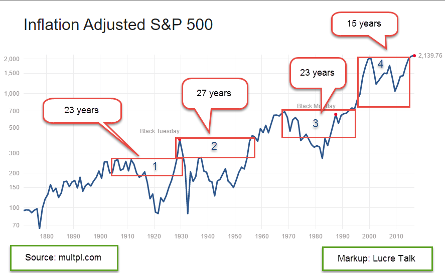
Unfortunately, the stock market road looks like Rt. 120 south of Mono Lake in California. The road is like a ribbon, marked by highs that are many years apart, more years than the majority of us will live in retirement.  In the graph from below from multpl.com I have marked up the decades-long periods before the inflation adjusted SP500 surpassed a previous high.  It is truly humbling.

It took 23 years for the market to finally surpass the high set in 1906.  Happy days!  Well, not quite.  Several months later came the stock market crash of 1929.  In 1932, the market fell near the 1920 lows.  In 1956, 27 years after the ’29 crash, the market finally notched a new high. In more recent decades, the market spent 23 years in a trough from 1969 to 1992.  Lastly, we have this most recent period from the high set in 2000 to a new high set in 2015.

IF – yes, the big IF – a person could call the high in a market, that would sure be nice, as Andy Griffith might say. (Youngsters can Google this.)  Of course, Andy would be suspicious of any city slicker who claimed to have such a crystal ball.  Knowing the high mark in advance is magic.  Knowing a previous high is not magic.

Looking at the chart we can see that the price in each period falls below the high of the period before it.  In the period marked “1” in the graph, the price fell below the high set in 1892. In period marked “2”, the price fell below the high set in 1906.  In the period marked “3”, the price fell below the high set in 1929.  In this last period marked “4” the price – well, it never fell below the high set in 1969.  The run up in the 1990s was so extreme that the market still has not truly corrected, according to some. Even the low set in 2008 didn’t come close to falling below the highs of that 1969-1992 period.  An investor who used a price rule that had been good for more than a hundred years found that the rule did not apply this time.

In 2008-2009, why didn’t prices fall below the high of the 1969-1992 period? They would have had to fall below 500 and in March 2009, there were a number of market predictors calling for just that. On March 9th, the SP500 index closed at 676, after touching a low of 666 that day.  The biblical significance was not lost on some. Announcements from major banks that they had actually been profitable in January and February caused a sharp rebound in investor confidence.  The newly installed Obama administration had promised some economic stimulus and the Federal Reserve added their own reassurances of monetary stimulus.

Did these fiscal and monetary relief measures prevent the market from fully purging itself?  Maybe.  Are stock prices wildly inflated because the Federal Reserve has kept interest rates so low for so long.  Could be.  How low are interest rates?  In 2013 the CBO predicted interest rates of 3-4% by this time.  They are still less than 1/2%.

How much are stock prices inflated?  Robert Shiller, the author of “Irrational Exuberance,” devised a price earnings ratio that removes most of the natural swings in earnings and the business cycle. Called the Cyclically Adjusted Price Earnings ratio, or CAPE, it divides the current price of the SP500 index by a ten year period of inflation adjusted earnings.  The current CAPE ratio is just below the high ratio set in 2007 by a market riding a housing boom.  The only times when the CAPE ratio has been higher are the periods during the housing bubble (2008), the dot-com boom (2000), and the go-go 1920s when many adults could buy stocks on credit.  Each of these booms was marked by a price bust that lasted at least a decade.

Price rules require some kind of foresight, and crystal balls are a bit cloudy.  There is a strong argument to be made for allocation, a balance of investments that generally are non-correlated, i.e. one investment goes up in price when another goes down.  An investor does not have to frequently monitor prices as with price rules. A once or twice a year reallocation is usually sufficient.

In an allocation strategy, equities and bonds are the most common investments because they generally counterbalance each other. A portfolio with 60% stocks and 40% bonds, or 60/40, is a common allocation. (Some people write the bond allocation first, as in 40/60.)   Shiller has recommended that an investor shift their allocation balance toward bonds when the CAPE ratio gets this high. For example, an investor would move toward a 60% bond, 40% stock allocation.

To see the effects of a balanced allocation, let’s look at a particularly ugly period in the market, the period from 2000 through 2011.  The stock market went through two downturns.  From 2000-2003, the SP500 lost 43% (using monthly prices). The decline from October 2007 to March 2009 was a nasty 53%.  In  2011 alone, a budget battle between the Obama White House and a Republican Congress prompted a sharp 20% fall in prices. During those 12 years, the SP500 index lost about 10%, excluding dividends.

During that period, a broad bond index mutual fund (VBMFX) more than doubled. Equities down, bonds up.  A rather routine portfolio composed of 60% stocks and 40% bonds had a total return of 3.75% per year.  Considering the stock market losses during that period, that return sounds pretty good. Inflation averaged 2.6% so that balanced portfolio had a real gain of about 1.2%.  Better than negative, we reason.  On the other hand, a portfolio weighted at 40% stocks, 60% bonds had a total annual return of 4.75%, making the case for Shiller’s strategy of shifting allocations.

There is also the nervousness of a portfolio, i.e. how much an investor gets nervous depending on one’s age and the various components of a portfolio.  During the 2000-2003 downturn in which the SP500 lost 43%, an investor with a 60/40 allocation had just 14% less than what they started with in the beginning of 2000. Not bad. 2008 was not pleasant but they still had 11% more than what they started with.  That is a convincing case for a balanced portfolio, then, even in particularly tumultuous times.

Can an investor possibly do any better by reacting to certain price triggers?  We already discussed one price rule that was fairly reliable for a hundred years till it wasn’t. The problem with rules are the exceptions and it only takes one exception to bruise an average 20 year retirement cycle.  Another price rule is a medium term one, the 50 day and 200 day averages.  These are called the Golden Cross and Death Cross.  Rules involve compromises and this rule is no exception.  In some cases, an investor may sell just when the selling pressure has mostly been exhausted.  Such a case was July 2010 when the 50 day average of the SP500 crossed below the 200 average, a Death Cross, and triggered a sell signal.  The market reversed over the following months and when the 50 day average crossed back above the 200 day average, a Golden Cross, an investor bought back in at a price 10% higher than they had sold!

The same scenario happened again in August 2011 – January 2012, buying back into the market in January 2012 at a price 10% higher than the price they sold at in August 2011.  These short term price swings are called whipsaws and they are the bane of strict price rules. In the past year there were two such whipsaws, one of them causing a 5% loss.  Clearly, this traditional trading rule needs a toss into the garbage can!  What works for a few decades may fail in a later decade.

For those investors who want a more active approach to managing a portion of their portfolio, what is needed is a flexible price rule that has been fairly reliable over six decades.  As a bull market tires, the monthly price of a broad market index like the SP500 begins to ride just above the two year average.  The monthly close will dip below that benchmark average for a month as the bull nears exhaustion.  If it continues to decline, that is a good indication that the market has run its course.  The price rule is an attention trigger that may not necessarily prompt action.

Let’s look at a few examples.  President Kennedy’s advisors were certainly aware of this pattern when the market fell below the two year mark in 1962.  They began pushing for tax cuts, particularly for those at the highest levels.  Rumors of a tax cut proposal helped lift the market back above the benchmark by the end of 1962   In early 1963, JFK made a formal proposal to lower personal rates by a third and corporate rates by 10% (At that time, corporations paid a 52% rate). An investor who sold after a two month decline suffered the same whipsaw effect, buying back into the market at about 10% higher than they sold.  However, at that selling point in 1962, rumors of tax cuts were helping the market rebound and might have caused an investor to wait another week before selling. The market had  in fact reached its low.

In mid-1966, the SP500 fell below its 24 month benchmark for seven months.  Escalating defense spending for the Vietnam War helped arrest that decline.

The bull market finally tired in the summer of 1969 and dropped below the 24 month benchmark in July.  The index treaded water just below the benchmark for a few months before starting a serious decline of 25%.  More than a year passed before the monthly price closed above the benchmark in late 1970.

The 1973 Israeli-Arab war and the consequent oil embargo threw the SP500 into a tailspin.  The price dipped below the average a few times starting in May 1973 before crossing firmly below in November 1973.  After falling almost 40%, the price finally crossed back above the benchmark in late 1974.  Remember that this was a particularly difficult fourteen year period marked by war, high unemployment and inflation, and a whopping four recessions.  The SP500 crossed below its ten year – not month, but year – average in 1970, again in 1974-75, and lastly in 1978.  Such crossings happen infrequently in a century and are great buying opportunities when they do happen.  To have it happen three periods in one decade is historic.

I’ll skip some minor events in the late 1970s and early 1980s.  In most episodes an investor can take advantage of these opportunities to step aside as the market swoons, then buy back in at a price that is 5-10% lower when the market recovers.

The most recent episodes were in November 2000 when the SP500 fell below its benchmark at about 1300. When it crossed  back over the benchmark in August 2003, the index was at 1000, a nice bargain.  This was another crossing below the ten year average.  The last one was in 2008 when the monthly price fell below the benchmark in January.  Although it skirted just under the average it didn’t cross back above the 24 month average.  In June it began a decline that steepened in September as the financial crisis exploded. Again the index fell below its ten year average. By the time the price closed back above the benchmark in November 2009, an investor could buy in at a 20% discount from the June 2008 price.

In September 2015 and again in February of this year, the index dropped briefly below its 24 month average. They were short drops but it doesn’t take much of a price correction because the index is riding parallel with the benchmark, above it by only 100 points, or less than 5%.  Corporate profits have declined for five quarters.  The bull is panting but still standing.

As we have seen in past exhaustions, there is a lot of political pressure to do something.  What could refuel the bull market? Monetary policy seems exhausted.  The Federal Reserve has indicated that they will use negative interest rates if they have to but they are very reluctant to do so.  Just this past week, the Bank of Japan (BOJ) indicated that their policy of negative interest rates is not helping their economic growth.  The BOJ had started down a negative interest rate path and has now warned other central banks not to follow.

What about fiscal policy? The upcoming election could usher in some fiscal policy changes but that seems unlikely.  Donald Trump has joined with Democrats advocating for more infrastructure spending but that is unlikely to pass muster with a conservative House holding the purse strings and a federal public debt approaching $20 trillion.  Only sixteen years ago, it was less than $6 trillion.  Democrats keep reminding everyone that the Federal Government can borrow money at very cheap rates.  However, the level of debt matters and Republicans will likely control the money in this next Congress.

Managing an entire portfolio with a price rule is a bit aggressive but might be appropriate for some investors who want to take a more active approach with a portion of their portfolio.  This price rule – or let’s call it guidance – is more a pain avoidance tool than a timing tool.

Timing Models

May 22, 2016

Long term moving averages can confirm the shifting trends of market sentiment and market watchers customarily watch for crossings of two averages.  The 50 week (1 year) average of the SP500 index just crossed below the 100 week (2 year) average, indicating a  broad and sustained lack of confidence.  Falling oil prices since mid-2014 have led to severe earnings declines at some of the large oil companies in the SP500.  The index is selling for about the same price as the two year average.

What to do?  These crossings or junctions can mark a period of some good buying opportunities – unless they’re not – and that’s the rub with indicators like this one.  Downward crossings typically occur after there has already been a 5 – 15% decline from a recent high.  If an investor sells some stocks at that time, they wind up selling at an interim low, and regret  their action when the market rises shortly thereafter.  They should have bought instead of sold.  AAAARGHHH, a false positive!  Twice in the 1980s, the sentiment shift was less than a year long and an investor who did act lost 10 – 20% as the market climbed after several months.

Conversely, after a 10-15% decline, some investors do buy more stocks, figuring that the excess optimism, or “fluff,” has been shaken out of the market.  Then comes that sinking feeling as the market continues to decline, and decline, and decline.  In April 2001 and July 2008, the 50 week average crossed below the 100 week average.  Investors who lightened up on stocks at those times saved themselves some pain and a lot of money as the broader market continued to lose another 30% or so.

There are not one but two problems with timing models: timing both the exit from and entry back into the market.  Over several decades the majority of active fund managers – professionals who study markets – did not get it right.  They underperformed a broad index like the SP500 because the index is actually a composite of the buying and selling decisions of millions of market participants.  John Bogle, the founder of the now gigantic Vanguard Funds, made exactly this point in his dissertation in the 1950s.  A half century later, this “wacky idea” of index investing has taken over much of the industry.

Consistently successful timing is very difficult and has tax consequences in some accounts.  Investors are encouraged to focus instead on their investment allocation to match their tolerance for risk and volatility, and to consider any prospective income that they might need from a portfolio.

Since 1960, the average annual price gain of the SP500 index has been 6.7%.  Add in an average yield (dividend) of 3% and the total return is almost 10% that an investor gains by doing nothing, a formidable hurdle for any timing model.

Within an allocation model, though, is the idea that an investor might shift a small portion of a portfolio from stocks to bonds and back in response to market signals.  In several previous articles I have looked at a Case-Shiller CAPE10 model (here, here, here, and here) as well as another crossing model using the 50 day and 200 day moving averages, dramatically named the Golden Cross and Death Cross (here, here, and here.)  As already mentioned, we want to avoid some of the false signals of crossing averages.

Instead of a crossing, we can simply use a change in direction of both averages.  When not just one, but both, long term averages turn down, we would move a portion of money from stocks to bonds, and in the opposite direction when both averages turned up.

Over the course of several decades, this strategy has been suprisingly successful.  The market sometimes experiences a decade when prices may be volatile but are essentially flat.  From 2000 – 2012 the SP500 index went up and down but was the same price at the beginning and end of that 12 year period.  1967 to 1977 was another such period, a stagnant period when an investor’s money would be better put to use in the bond market rather than the stock market.

In recent decades, this long term weekly model would have favored stocks from 1982 to March 2001 while the market gained 850%, an annual price gain of 11%.  The model would have shifted money back to stocks in August 2003 at a price about 25% less than the exit price in March 2001. In March 2008, the model would have favored an exit from stocks to bonds.  The stock market at that time was about the same price that it had been 7 years earlier in March 2001.  The model captured a 30% gain while the index went nowhere.

In the 1967 – 1977 period, the model did signal several entries and exits that produced a cumulative 8% price loss over the decade but the model favored the bond market for half of that period when bonds were earning 8% per year, a net gain.

In almost two years, the SP500 has changed little; the yield is less than 2%, far lower than the 3% average of the past 50 years.  However, the broader bond market has also changed little in that time and is paying just a little over 2%.  There are simply periods when strategies and alternatives have little effect. Although the 50 week average crossed below the 100 week average earlier this month, they are essentially horizontal.  The 100 week average is still rising, but barely so, a time of drift and inertia.  In hindsight, we may say it was the calm before a) the storm (1974), or b) the surge (1995). Usually the calm doesn’t last more than two years so we can expect some clear direction by the end of the summer.

/////////////////////////////

It’s the economy, stupid!

One of the myths of Presidential politics is that Presidents have a lot to do with the strength or weakness of the economy, a superhero narrative carefully cultivated by the two dominant parties.  Here’s a comparison of GDP growth during Democratic and Republican administrations. The Dems have it up on the Reps since 1928, chiefly because the comparison starts near the beginning of the Great Depression when the Reps held the Presidency.

For several reasons, GDP data is unreliable during the Depression and WW2 years.  First, the GDP concept wasn’t formalized till just before the start of WW2 so data collection was new, primitive and after the fact.  Secondly, this 14 year period includes an extraordinary amount of government spending which warped the very concept of GDP.  The WPA program that put so many to work during the depression years was a whopping 7% of GDP (Source), like spending $2 trillion dollars, or half the Federal budget, in today’s economy.

The Federal Reserve begins their GDP data series after WW2 when data collection was much improved. If you’re a Dem voter, don’t mention this unreliable data.  Just tell friends, family and co-workers that the Dems have averaged 4% GDP growth since 1927; the Reps only 1.7%.  If you’re a Republican voter, exclude the 20 year period from 1928 to 1947 and begin when the Federal Reserve trusts the data. Starting from 1947,  Republicans have presided over economies with 2.75% annual growth during 36 Presidential years.  During the 30 years Dems have held the Presidency, there has been a slighly greater growth rate of 3.1%.

In short, economic growth is about the same no matter which party holds the Presidency.  Shhhh! Don’t tell anyone till after the election is over.  Legislation by the House and Senate has a much greater impact on the economy.

///////////////////////////

Small Business

“If America is going to dominate the world again, the country has to fix the spirit of free enterprise. Small-business startups are in serious decline.”

“Gallup finds that one-quarter of Americans say they’ve considered becoming business owners but decided not to. ”

These foreboding quotes are from a recent Gallup poll.  Small businesses employ more than 50% of employees and are responsible for the majority of job growth yet many politicians and most voters pay little attention to the concerns of small business owners.  The giant corporations get most of the press, praise and anger.  Could the lack of small business growth be responsible for the lackadaisical growth of the entire economy during this recovery?  As the population  continues to age, growth will be critical to fund the dedication of community resources to both the old and young.

The BLS routinely tracks the Employment-Population Ratio, which is the percentage of people over 16 who are working, currently 60%.  But this ratio does not fully capture the total tax pressures on working people since it excludes those under 16, who require a great deal of community resources.  When we track the number of workers as a percent of the total population, we see a long term decline.  As this ratio declines, the per-worker burdens rise for it is their taxes that must support programs for those who are not working, the young and the old.

Regulatory burdens hamper many small businesses. A recent incident with a Denver brewery highlights the sometimes arbitrary rulemaking that business owners encounter.  Agencies protest that their mission is to ensure public safety.  An unelected manager or small committee in a department of a state or local agency may be the one who decides what is the public safety.  As the rules become more onerous and capricious, fewer people want to chance their savings, their livelihood to start a small business.  As fewer businesses start up, tax revenues decline and the debate grows ever hotter: “more taxes from those with money” vs “less generous social programs.”  Policy changes happen at a glacial pace, further exacerbating the problems until there is some crisis and then the changes are instituted in a haphazard fashion. Since we are unlikely to change this familiar pattern, the issues, anger and contentiousness of this election season are likely to increase in the next decade.  Keep your seat belts buckled.

Year End Approaches

December 19, 2015

For those of you who pay attention to crossing averages, the 50 day average of the SP500 index just crossed above the 200 day average.  This long term buy signal is often referred to as the Golden Cross.  The Death Cross, when the 50 crossed below the 200 day average in early August, is a sell signal.  Those who sold some of their holdings at that time missed the volatility of the past few months.  The index was at 2100 in early August.  It closed at approximately 2000 on Friday.  The index has lost about 4% in the past two days.

Past buy crosses were June 2009, October 2010, January and August 2012 and this past week.  Recent sell crosses were December 2007, July 2010, August 2011, July 2012, and August 2015.

In buy, sell order they were December 2007 (sell), June 2009 (buy), July 2010 (sell), October 2010 (buy), August 2011 (sell), January 2012 (buy), July 2012 (sell), August 2012 (buy), August 2015 (sell) and December 2015 (buy).  Note the three year period between buy and sell signals from August 2012 to August 2015.  The market gained 55% during that period.

As you can see from the list above, the market usually regains its footing after a few months – except when it doesn’t, as in 2008.  This buy sell rule avoided the protracted market downturns in 2000 and 2008 at the expense of acting on signals that are false positives, or what is known in statistics as Type I errors.

*****************************

Cost Basis

Mutual fund companies typically calculate an investor’s cost basis for their funds.  Some investors mistakenly think that cost basis reflects the performance of their investment.  It doesn’t. Let’s look at an example of a cost basis entry:

At first glance, an investor might think they have lost $186 since they first started investing in the fund.  Usually, that’s not the case.  In this case, the fund has earned more than $5000 in ten years.

Let’s look at some basics.  An investor in a mutual fund has the option of having dividends and capital gains reinvested in the same fund or transferred to another fund like a money market.  To begin our simple example, let’s choose to NOT reinvest.

Let’s say an investor put $1000 in a bond fund BONDX.  Each share sells for $100 so they have bought 10 shares.  Every quarter the fund pays a $1 dividend per share.  A day before the dividend is paid the fund’s share price is $101.  The fund then distributes the $1 dividend.  The market value of each share instantly falls by the amount of the dividend – $1 – so that after the dividend the market value of each share of BONDX is $100.  What is the investor’s cost basis?  $1000.  The market value is 10 shares x $100 = $1000.  Capital gain or loss? $0.  Does this mean the investor has made no money?  No, they have an extra 10 shares x $1 dividend per share = $10 in their money market account.

When opening up a fund the default option may be to reinvest capital gains and dividends.  This is where some investors get confused.  So, let’s change the reinvest option and choose YES. Now, as before, the fund distributes the $1 dividend and the share price of the fund falls to $100, just as before.  Now, however, the money is not transferred to the money market fund.  Instead it is used to buy more shares of BONDX.  The $10 that the investor receives buy a 1/10 share of BONDX.  Now the investor owns 10.1 shares of BONDX at a cost of $100 per share = $1010 cost basis.  The market price of the fund is $100 per share x 10.1 shares = $1010.  Captial gain or loss: $0.  Again, the capital gain or loss does not reflect the total performance, or profit and loss, of the investment.  The profit is $10.

So, the capital gain or loss should be used only to calculate the tax effect of selling a fund, not the performance of the fund.  The fund company will calculate the performance, or the rate of return (IRR) on an investor’s funds on a separate screen.  Choose that option instead of the cost basis screen.

******************************

The Investment Cycle

Investments tend to rise and fall in price over the course of a business cycle.  At the end of an expansionary cycle, commodity prices start falling.  Yardeni Research has some good graphs which illustrate the ongoing plunge in commodity prices.

As the economy begins its contraction phase, the prices of bonds start to fall.  As we enter recession or at least a contraction of growth, stocks fall.  In the recovery, comodities rise first, followed by bonds, then stocks.  Here is more information for readers who are interested in exploring the details and background of this cycle.

***************************
Diabetes

The American Diabetes Assn puts the direct costs of treating diabetes at $150 billion.  That is 25% of the $600 billion spent on Medicare in 2014.  Indirect costs add another $75 billion in costs.  Much of the increased expenditure is for treating late onset Type II diabetes.  Expenses are sure to grow as the population ages and people do not make the life style changes needed to delay or moderate the onset of the disease.

***************************
Credit Spreads

Several weeks ago, I noted the growing “spread” between Treasury bonds and high yield junk bonds.    The graph I showed was the benchmark of junk bonds, the Master II class. Let’s call them Bench Junks. The bottom of the barrel, so to speak, are those company bonds rated CCC and lower.  These are companies that are more likely to default as economic growth slows or contracts. Let’s call them Low Junks. While the Bench Junks’ spread shows investor concern, the Low Junks’ spread shows a stampede out of these riskier bonds.  A rising spread means that the prices for those bonds are falling, effectively giving buyers a higher interest rate. Investors want the higher yield to compensate them for the higher risk of owning the bonds.

Here is an article explaining the composition of some high yield bond ETFs for those readers who are interested. in learning more.

**************************

Income Taxes

Turbo Tax may be the most widely used individual income tax software but there are many providers of tax software.  Each state usually lists the software programs it has approved.  You can Google “approved income tax software” and insert your state name at the beginning of the search term. Here is a link to Colorado‘s list of approved software.  Here is the list for Texas, New York and California.

**************************
Lastly, have a wonderful Christmas!

A Bull In A China Shop

August 16, 2015

The big news this week was China’s decision to devalue its currency, the yuan, by 3.5% in two days.  At week’s end, the yuan was about 3% less than what it was at the start of the week.

The decline in value came abruptly in  a market that moves in hundredths of a percent, called basis points, each day.  Since the beginning of the year, the euro has lost more than 8% against the dollar but it has done so in little teeny tiny moves.

What prompted China’s central bank to make this devaluation?  China expected a small drop in exports in July, but 8% was far more than expected. (Bloomberg )  The timing of the devaluation couldn’t be worse.  Emerging markets in southeast Asia have had sluggish growth in the past year and depend on exports.  The devaluation of the Yuan makes Chinese exports more competitive.  Vietnam and Malaysia devalued their currencies this week to maintain a competitive edge with China.

Emerging markets have had a rough ride this year.  A popular Vanguard Emerging Markets ETF is down 18% from its high in April.  However, today’s price level is barely below the price in mid-December.

While the SP500 has gone nowhere for the past nine months, emerging markets went on a tear in the beginning of the year, rising about 20% before falling back.  Talking about the SP500…

Dow Jones Death Cross alert!!! This past week the 50 day moving average of the Dow Jones Index crossed below the 200 day average.  The sky is falling.  Run for the hills.  The rhetoric does get a bit dramatic.  Should an investor disregard this signal as so much hocus-pocus?  Brett Arends at MarketWatch suggests that this “indicator” is hogwash. Yes and no.  The Dow Jones is a narrow index composed of just 30 stocks (CNN Money on component performance YTD).  Although it is meant to capture the essentials of the U.S. market, its narrowness makes it an unreliable indicator in some environments.  The oil giants Chevron and Exxon have dropped 23% and 15% respectively, dragging the index down.  There has still not been a death cross in the broader SP500 index.

To investors now over 60, the equity markets of the past 15 years have told a sobering message.  Investors need to either pay some attention or pay someone to pay some attention.  The SP500 stock market index has only recently recovered the inflation adjusted value that it had in 2000.

In nominal, or current, dollars, recoveries from major price declines can often take seven years.  Past recovery periods were 1968 – 1972, 1973 – 1980, 2000 – 2007, and 2007 to early 2013.

Long term trending indicators may be able to help an investor avoid some – emphasize some – of the pain.  For the casual investor, a death cross is a signal to pay a bit more attention to the market on a weekly basis.  All death crosses are not created equal.  Some death crosses are wonderful buying opportunities.  In July 2010, after a two month drop of almost 20%, the 50 day average of the SP500 dropped below the 200 day average, a death cross.  Good time to buy.  Why?  Because it is a death cross coming after a sharp recent drop in price.  The same type of death cross occurred in August 2011 after a steep drop in stock price in late July after the “budget battle” between Obama and Boehner went unresolved.  Good buying opportunity.

In December 2007, a death cross was not a good buying opportunity?  Why?  Because it came after six months of the market seesawing with indecision and no net change in price.  That indicates that there is a shifting sentiment, a lack of confidence among investors.

Some mid-term to long-term strategists use a weekly chart which measures the price at the end of each week, that price that short term traders feel comfortable with as they head into the weekend.  In a bullish or positive market the 12 week, or 3 month, price average stays above the 50 week, or one year, average.  As indecision creeps in the two averages will get close.  Finally, the 50 week average will top out, either gaining nothing or losing just a tiny bit as the 12 week average crosses below.  We’re not there.  We may get there.  Who knows?

Once that weekly cross happens, a long term investor might look at a daily chart.  What is a good rule(s) of thumb to determine whether a death cross is a good buying opportunity, a negative signal, or a palms up, who knows what the heck is going on, signal?

1) Has there been a decline of 15 – 20% (high price to low price) in the past 2 – 3 months? Is today’s price several percent below the 50 day average? Then it is probably a good buying opportunity as I noted above.  It is not always clear cut.  In September 2000, the SP500 began a 12% slide in price that would mark the beginning of a downturn lasting several years.  In mid-October 2000 a death cross occurred.  Was that a large enough slide in price to present a good buying opportunity?  Not really.  The price that day was almost the same as the 50 day average.  The recent drop in price had contributed to the death cross but a longer term re-evaluation of value was also taking place that would cut the SP500 index by 45% toward the end of 2002.

2) If there has been no substantial decline in the past few months, look at the closing price on the day of the death cross.  How many months can you go back to find the same price level and how many times has that price level been tested?  If just a few months, then this is an indeterminate period of indecision that may resolve itself.  Prices may move either higher or lower depending on the resolution.  But, if you can go back six to nine months of price flipping and flopping, then it is a bit more serious.  There may be a spreading questioning of value, a re-positioning of asset balances.  Does it mean sell tomorrow?  No.  It means pay attention.

After several years of declining prices in the years from 2000 – early 2003, the market had a Golden Cross (50 day average rises above 200 day) in May of 2003.  A death cross occurred more than a year later, in August 2004, at the 1095 price level.  That day’s price was close to the 50 day and 200 day average and so was not a standout buying opportunity. The market had first crossed above that price level in December 2003, then retested that level three times on market declines only to rise again.  Might it have been worth waiting a few weeks to check the market’s short term sentiment and see if that price level would hold again?  Probably. As it turned out, the market continued to rise for three more years.

These are not ironclad rules but act as guidelines to help an investor gauge the underlying mood of the market to make more informed investing decisions.

Trends and Bubbles

November 17, 2013

This week the department store Macy’s reported sales growth that was above forecast.  Same store sales rose 3.5%, about 50% better growth than expected.  Macy’s attracts a higher income customer than Target, J.C. Penney or Wal-Mart.  On Thursday, Wal-Mart announced that their sales had declined for a third quarter in a row.  The holiday season depends on lower and middle working class folks, the kind who shop at Wal-Mart, to open their pockets.  Investment firm Morgan Stanley expects this retail season to be the worst since 2008 when the country was deep in recession. (Source)
What can we learn from a bird’s eye view of the growth in consumer credit?  At 5.6% year over year, it is stable.

Note the response time lag in this series.  The growth in consumer credit did not decline below 5% till months after the recession started.  Despite the loss of hundreds of thousands of jobs in the beginning of 2008, this net job loss represented less than 1% of the work force in mid-2008.  The job loss would mount into the millions but jobs are “sticky,” meaning that a downturn in the economy has a minor effect on most people most of the time.  After the fact, it is easy for us to point at some chart, arch our eyebrows in a knowing glance, and say “We can see the breakdown of the economy beginning here.”

On a long term chart, we can see a reduction in growth swings over the past thirty years.  Relatively flat income growth for a majority of workers has dampened the swings.  While good for household balance sheets, it means that we can expect less economic volatility but also muted growth for the next decade.

Expectations for the holiday season are not reflected in the price of retail stocks.  A basket of retail companies has grown about 40% this year and is up about 70% over two years.  It may be time to take a bit off the table in this sector.

The Consumer Financial Protection Bureau (CFPB) was created a few years ago to act as a watchdog over the credit practices of the largest banks.  On Tuesday, Richard Cordray, Director of the agency appeared before a Senate committee.  He confirmed that the agency collects a lot of anonymized data on 900 million credit card accounts each month as part of its supervisory role.  Questions should be raised whenever any government agency collects data on us.  How is the data protected?  Who has access to the data?  What about my privacy?

Mr. Cordray noted that several other agencies as well as private industry collect this data.  Because the data is anonymized, we are little more than a number to  the agency, but there are several concerns.  Federal agencies have a great deal of legal power, enabling them to get a warrant to access  the data on anyone.  Cordray repeatedly assured the committee that no one at the agency is interested in our personal data but left off one adverb – “now.”  In the aftermath of 9-11, anti-war protestors found themselves turned away at airports or flagged for additional screening.  How did federal agencies know the travel plans of many protestors?  It does not take a team of FBI agents to trace the activities of any citizen when several federal agencies have our monthly financial activity at their fingertips.  Secondly, there is the matter of security.  How many parties does our data go through on its way to the agency?  Where and at what stage in the process of data aggregation is the anonymizing done?  Is our personal credit card info transmitted first to a separate third party anonymizer before being transmitted to the various agencies?  Is the raw data being transmitted to an agency which then anonymizes the data using a third party program or process?  In any case, it was clear that our monthly card transactions are making the rounds in both private industry and various government agencies.

The stock market continues to rise, prompting talk of a bubble.  If you have access, try to read “Is This A Bubble” by Joe Light in this weekend’s edition of the Wall St. Journal.   It is both informative and measured in its assessment.

 In February 2012, I mentioned the Golden Cross which had occurred in late January.  This long term indicator of market sentiment is a crossing of the 50 day moving average of stock market prices above the 200 day average.

Since then the market has risen about 40%.  Man, if I had only taken my own advice and moved all my investments and money into the stock market!  As the market continues to rise, more and more investors catch the “if only” disease and start moving money from safer investments into stocks.  This is why many of us tend to buy high and sell low.  Instead we should stay with the fundamentals of diversify, diversify, and lastly – diversify.  A long term indicator like the Golden Cross is not a signal to dump all of our savings into stocks – unless we are in our 30s and have lots of time before we need the money.  A more sensible approach is to adjust allocation upwards towards stocks and this depends on a person’s age, needs, and fears.  If a person has a 50% stock allocation, with the remaining 50% in bonds and cash (I’ll leave alternate investments out for right now), that indicates a moderate tolerance for risk.  They might shift the allocation to 55% stocks or 60% when they see a Golden Cross.   A person who has a 70% allocation to stocks, indicating a high tolerance for risk, might start adjusting to an 85% to 90% allocation.  Using this more moderate approach, a person would have lightened up their stock allocation in December 2007 when a reverse Golden Cross happened.

So what if someone has been very scared of the stock market and has only 10% of their savings in stocks?  Should they move some money into the market now?  That depends.  If the thought of making even a slight change leads a person to lose sleep, then no.  Should someone change their allocation of stocks from 10% to 50% now?  That is a major allocation change and should be done using dollar cost averaging.  This is a process where one takes money from one investment basket every month and puts it in another investment basket. There is also a psychological advantage to this approach.  As a person’s allocation percentage becomes a bit riskier, they can adjust to the additional risk in a measured way.

Tolerance for risk is a composite of several components:  psychological or emotional, future liquidity needs, age, and assets as well as income sources.  Too often, people think of tolerance for risk as an emotional response only.  While it is true that our emotions can cloud our measured response to risk, it is important to keep in mind that it is only one of the components.

**************

In answer to calls from his own party members, President Obama announced an administrative change to the Affordable Care Act (ACA) that allows those with policies in the individual health care market to retain their policies even if the policies don’t meet the minimum standards of the ACA.  Politicians, pronouncements and podiums – stir them together and voila!  The President’s pronouncement was little more than political cover at this late stage in the transition to Obamacare.  Only if the states allow it and companies decide to offer the plans will an individual policy holder be able to “keep their plan,”  as the President promised on numerous occasions in the past few years.

On Friday, the Energy and Commerce Committee released emails subpoenaed from CMS, the agency that administers Medicare and the ACA.   The emails contradict previous testimony by both CMS head administrator Marilyn Tavenner and HHS Secretary Kathleen Sibelius that only routine problems with the healthcare.gov web site were anticipated before the launch of the web site.  Ms. Tavenner testified that there were enough problems that they decided to delay the implementation of the small business plans on the web site but it appears that the problems went much further and top officials were alerted.

Henry Chao, the deputy CIO at CMS, was made aware of many major security, transactional and design problems with the web site during the summer but decided – or was pressured to decide – that the site would go live on October 1st regardless.  President Obama’s repeated selling point has been what he calls “smart” government. The rollout of the federal health care website has  revealed – once again – that the government in Washington has become too big and too top down to be smart, or effective.  To keep their campaign coffers filled, too many in Washington must placate those companies which fund those coffers, including special favors and bailouts for the elite on Wall Street.  To get the votes, they must placate the poor with programs and promises.

A conflict of interests and a clash of incentives makes most of the Washington crowd ineffective.  Turn on C-Span and watch the faces of the House and Senate Budget Conference (House and Senate).  These are intelligent, committed people who feel the pull of these different puppet masters, those political interests that keep them in their respective seats.   Each one of them earnestly wants to fix the problem – and that is the problem.  Much of the time, they are fixing the previous fixes they implemented.  This approach makes Congress feel important. I would suggest that they do little more than enact incentives and let their constituents craft the solutions.  Sure, the solutions will not be crafted with the superior technical expertise that Washington promises. Instead, they will emerge in a stumbling, hodge-podge way that will disenchant those who believe in the romantic notion of omniscient experts who engineer elegant solutions to social and economic problems.  I hope that one day the Washington elite will let Main St. try to figure out the solutions to some of these problems. We can do better.