A Home Is a Magic Wallet

April 7, 2024

by Stephen Stofka

In this week’s letter I will explore the various roles that housing plays in our lives. Last week I showed the divergence of household formation and housing supply during the financial crisis. Home builders responded to the downturn in household formation by building fewer homes. Because the recovery after the crisis was slow, the demand for housing did not pick up until 2014. It is then that a mismatch between housing demand and supply started to appear in the national and some local home price indices. This week I will examine the demographics of homebuyers and sellers in recent history and the secret life of every homeowner as a landlord. A home is a magic wallet where money flows come and go.

Data from the National Association of Realtors (NAR) indicates that the median age of home sellers has increased from 46 to 60 since 2009. I will leave NAR data sources in the notes. In the four decades between 1981 and 2019, the median age of home buyers rose by twenty years, from 36 in 1981 to 55 in 2019. The median age of first-time buyers, however, increased by only four years, from 29 to 33. In 1981, the difference in age and accumulated wealth between first-time buyers and all buyers was only seven years. Now that difference has grown to 22 years. First-timers typically buy a home that is 80% of the median selling price of all homes.

In the past four decades, there has been a divergence in wealth between older and younger households. The real wealth of younger households has declined by a third since 1983 while households headed by someone over 65 have enjoyed a near doubling of their real wealth in thirty years. Accompanying that imbalance in growth has been a shift in capital devoted to housing.

The Federal Reserve regularly updates their estimates of the changes in household net wealth. The link is an interactive tool that allows a user to modify the time period of the data portal. The chart below shows the most recent decade of changes in wealth. The lighter green bars are the changes in real estate wealth for households and non-profits and show the large gains in real estate valuations during the pandemic. The blue bars represent equity valuations and demonstrate the volatility of the stock market in response to any crisis, large or small.

The Fed’s data includes various types of debt as a percent of GDP. Twenty years ago, household mortgages were 11-12% of GDP. Today they are 19% of GDP, a huge shift in financial commitment to our homes and neighborhoods. A city average of owner equivalent rent (FRED Series CUSR0000SEHC) averaged an annual gain of 2% during Obama’s eight- year term, 2.8% during Trump’s term, and 6% during the first three years of Biden’s term. Biden has little influence on trends in housing costs, but the art of politics is to use correlation as a weapon against your opponent. People feel the change in trajectory as a burden on their households.

The Bureau of Labor Statistics calculates owner equivalent rent by treating a homeowner as both a landlord and renter. Property taxes, mortgage payments, interest, maintenance and improvements to a home are treated as investments just as though the owner were a landlord. The BLS uses housing surveys to determine the change in rental amounts for different types of units. A sample of homeowners are asked how much they would rent out their home but this guess is used only to establish a proportion of income dedicated to rent, not the actual changes in the rental amounts for that area, as the BLS explains in this FAQ sheet.

Let us suppose that a homeowner has a home that is fully paid for. If the house might rent for $2000 a month and monthly expenses are $500 a month, that would represent $1500 per month in implied net operating income for that homeowner, an annual return of $18,000. A cap rate is the amount of net operating income divided by the property’s net asset value. If similar homes are selling for $450,000 in that area, the homeowner is making 4% on their house’s asset value, slightly less than a 10-year Treasury bond (FRED Series DGS10, for example).

Long-term assets compete with each other for yield, relative to their risk. A property is a riskier investment than a Treasury bond, so investors expect to earn a higher yield from a property. Before the pandemic, 10-year bonds were yielding between 2-3%. Landlords could charge lower rents and still earn more than Treasury bonds. As yields rose for Treasury bonds, property investors must charge higher rents to earn a yield appropriate to the risk or sell the property and invest the money elsewhere.

When we own an asset that provides an income, it is as though the asset owes us. When a home declines in value, we feel a sense of loss. When the housing market turned down in 2007-2008, homeowners expected to get a similar price as the house their neighbor sold in 2006. They used that sale price to determine what their house owed them. In order to get the listing, a real estate agent would agree to list the home for that higher amount, but the property would get few offers. After a period of time, the seller would cancel the listing and wait for the “market to turn around.”

Earlier I noted the dramatic rise in mortgage debt as a percent of GDP. At one-fifth of the economy, that debt represents capital that is not being put to its most efficient use because most homeowners do not regularly evaluate the yield on their homes as professional investors. A higher percent of capital devoted to housing will help sustain higher housing costs and pressure household budgets. I worry that an inefficient use of capital will contribute to a pattern of lower economic growth in the future, stifling income growth. The combination of these two pressures will make it difficult for younger households to thrive. The generational gap will widen, adding more social and political discord to our national conversation.

/////////////////

Photo by Towfiqu barbhuiya on Unsplash

Keywords: mortgage, housing, owner equivalent rent

Notes on median age of sellers: 2009 data is from the NAR and cited in a WSJ article (paywall). Current data is from the NAR FAQs sheet. Jessica Lautz, an economist with NAR, reported the four-decade trend in home buyers. Median home prices of first-time buyers is from a 2017 analysis by the NAR. The comparison of older and younger households comes from a 2016 NAR analysis.

Notes on Federal Reserve data:  The change in mortgage debt as a percent of GDP is in the zip file component z1-nonfin-debt.xls, in the column marked “Noncorporate Mortgages; Percent of GDP.”

The Role of a Rule

December 31, 2023

by Stephen Stofka

This week’s letter is about the role of a monetary rule and the guiding points that help the Fed steer its policymaking. Since the 2008-9 financial crisis, the Fed has purchased a lot of assets, increasing its balance sheet from less than one trillion dollars at the end of 2007 to almost $8 trillion this month. It has kept the federal funds rate that anchors all other interest rates near zero for ten of the last 15 years. The members on its board of governors serve 14 year terms, affording them an autonomy resistant to political influence. From those board members the President and Senate choose and confirm the Chair and Vice-Chair of the board. The governance structure allows them to set and follow a plan of steady guidance but their actions have resembled those of sailors steering against unpredictable winds. What are the guiding lights?

In the late 1950s, economists and policymakers enthusiastically endorsed the concept of the Phillips Curve. Picture an ellipse, a circle that has been stretched along one axis so that it appears like an egg.

Think of unemployment along the x-axis and inflation along the y-axis. More unemployment stretched the circle, shrinking inflation. More inflation stretched the circle in the y-direction, lessening unemployment. Policymakers could tweak monetary policy to keep these two opposing forces in check. In the 1970s, both inflation and unemployment grew, shattering economic models. Nevertheless, Congress passed legislation in 1978 that essentially handed the economic egg to the Fed. While the central banks of other countries can choose a single policy goal or priority – usually inflation – Congress gave the Fed a twin mandate. It was to conduct monetary policy that kept inflation steady and unemployment low – to squeeze the egg but not break it.

Mindful of its twin mission, the Fed later recognized – rather than adopted – a monetary policy rule, often called a Taylor rule after John B. Taylor (1993), an economist who proposed the interest setting rule as an alternative to discretion. The Fed would use several economic indicators as anchors in policymaking. The Atlanta Fed provides a utility that charts the actual federal funds rate against several alternate versions of a Taylor rule. I’ve included a simple alternative below and the actual funds rate set by the Fed. When the rule calls for a negative interest rate, the Fed is limited by the zero lower bound. Since the onset of the pandemic in March 2020, the Fed’s monetary policy has varied greatly from the rule. Only in the past few months has the actual rate approached the rule.

In a recent Jackson Hole speech, Chairman Powell said, “as is often the case, we are navigating by the stars under cloudy skies.” What are these guiding points that should anchor the Fed’s monetary policy? I’ll start with r-star, represented symbolically as r*, which serves as the foundation, or intercept, of the rule. Tim Sablick at the Richmond Fed defined it as “the natural rate of interest, or the real interest rate that would prevail when the economy is operating at its potential and is in some form of an equilibrium.” Note that this is the real interest rate after subtracting the inflation rate. The market, including the biggest banks, consider it approximately 2% (see note at end). This is also the Fed’s target rate of inflation, or pi-star, represented as π*. The market knows that the Fed is going to conduct monetary policy to meet its target inflation rate of 2%.

Why does the Fed set a target inflation rate of 2% instead of 0%? The Fed officially set that target rate in 1996. The 2% is a margin of error that was supposed to give the Fed some maneuvering room in setting policy. There was also some evidence that inflation measures did not capture the utility enhancements of product innovation. Thirdly, if the public expects a small amount of inflation, it adjusts its behavior so that the cost is so small that the benefit is greater than the cost (Walsh 2010, 276). Today, most central banks set their target rate at 2%.

The definition of r-star above is anchored on an economy “in some form of equilibrium.” How does the Fed gauge that? One measure is the unemployment rate and here we have another star, U-star, often represented as un, meaning the natural rate of employment. In 1986 Ellen Rissman at the Chicago Fed described it (links to PDF) as “the rate of unemployment that is compatible with a steady inflation rate.” So now we have both unemployment and the interest rate anchored by the inflation rate.

Another part of that r-star definition is an economy “operating at potential.” Included in the Fed’s interest rate decisions is an estimate of the output gap that is produced by economists at the Congressional Budget Office (CBO). The estimate includes many factors: “the natural rate of unemployment …, various measures of the labor supply, capital services, and productivity.” The CBO builds a baseline projection (links to PDF) of the economy in order to forecast the federal budget outlook and the long term financial health of programs like Social Security. Each of these factors does contribute to price movement but the analysis is complex. A more transparent gauge of an output gap could help steer public expectations of the Fed’s policy responses.

In a paper presented at the Fed’s annual Jackson Hole conference in Wyoming, Ed Leamer (2007, 3) suggested that the Fed substitute “housing starts and the change in housing starts” for the output gap in constructing a monetary policy rule. At that time in August 2007, housing starts had declined 40% from their high in January 2006. Being interest rate sensitive, homebuilders had responded strongly to a 4% increase in the Fed’s key federal funds rate. Despite that reaction, the Fed kept interest rates at a 5% plateau until September 2007. By the time, the Fed “got the message” and began lowering rates, the damage had been done. Six months after Leamer delivered this paper, the investment firm Bear Sterns went bankrupt. The Fed engineered a rescue by absorbing the firm’s toxic mortgage assets and selling the rest to JP Morgan Chase. Six months later, Lehman Brothers collapsed and the domino effect of their derivative positions sparked the global financial crisis.

I have suggested using the All-Transactions House Price Index as a substitute for the output gap. A long-term average of annual changes in this index is about 4.5%. The index is a summation of economic expectations by mortgage companies who base their loan amounts on home appraisals, banks who underwrite HELOC loans to homeowners and loans to homebuilders. The index indirectly captures employment trends among homeowners and their expectations of their own finances. Any change that is more than a chosen long-term average would indicate the need for a tightening monetary policy. Anything less would call for a more accommodative policy. Either of these housing indicators would be a transparent gauge that would help guide the public’s expectations of monetary policy.

Although the Fed considers the Taylor rule in setting its key interest rate, the rate setting committee uses discretion. Why have a rule only to abandon it in times of political or economic stress? The rule may not operate well under severe conditions like the pandemic. A rule may be impractical to implement. A Taylor rule variation called for a federal funds rate of 8% in 2021. This would have required a severe tightening that forced the interest rate up 7% in less than a year. The Fed did that in 1979-80 and again in 1980-81. Both times it caused a recession. The second recession was the worst since the 1930s Depression. An economy as large as the U.S. cannot adjust to such a rapid rate increase.

How strictly should a rule be followed? Some of us want rule making to be as rigid as lawmaking. A rule should apply in all circumstances regardless of consequences. Many Republican lawmakers felt that way when they voted against a bailout package in September 2008. Some of us regard a rule as an advisory, not a straitjacket constraint of policy options. Each of us has a slightly different preference for adherence to rules.

See you all in the New Year!

/////////////

Photo by Mark Duffel on Unsplash

Keywords: housing starts, house price index, stars, output gap, unemployment, interest rate, inflation

All-Transactions House Price Index is FRED Series USSTHPI. The annual change is near the long-term average of 4.5%, down from a high of 20% in 2022.

Housing starts are FRED Series HOUST. The output gap is a combination of two series, real GDP GDPC1, and real potential GDP, GDPPOT.

A gauge of long-term inflation expectations is the 10-year breakeven rate, FRED Series T10YIE. The 20-year average is 2.08%. The series code is T=Treasury, 10Y = 10 year, IE = Inflation Expectations. The T5YIE is a 5-year breakeven rate.

Leamer, E. (2007). Housing Is the Business Cycle. https://doi.org/10.3386/w13428

Taylor, J. B. (1993). Discretion versus policy rules in practice. Carnegie-Rochester Conference Series on Public Policy, 39, 195–214. https://doi.org/10.1016/0167-2231(93)90009-l

Walsh, C. E. (2010). Monetary theory and policy. MIT press.

Housing Heats Up

June 5, 2016

In parts of the country, particularly in the west, demand for housing is strong, causing higher housing prices and lower rental vacancy rates.  For the first quarter of 2016, the Census Bureau reports that vacancy rates in the western U.S. are 20% below the national average of 7.1%.  At $1100 per month, the median asking rent in the west is about 25% above the national average of $870 (spreadsheet link).

With a younger and more mobile population, home ownership rates in the west are below the national average (Census Bureau graph). Housing prices in San Francisco have surprassed their 2006 peaks while those in L.A.are near their peak.  Heavy population migration to Denver has spurred 10% annual home price gains and an apartment vacancy rate of 6% (metro area stats).

From 1982 through 2008, the Census Bureau estimates that the number of homeowners under age 35 was about 10 million. These were the “baby bust” Generation X’ers who numbered only 70% of the so-called Boomer generation that preceded them.

Shortly before the financial crisis in 2008, a new generation came of age, the Millenials, born between 1982 and 2000, and now the largest age group alive in the U.S. (Census Bureau). Based on demographics, homeownership should have increased to about 13 million in this younger age group, but the financial crisis was particularly hard on them.  Starting in 2008, homeownership in this younger demographic began to decline, reaching a historic low of 8.8 million in 2015, a 15% decline over seven years, and a gap of almost 33% from expected homeownership based on demographics.

In response to lower homeownership rates, builders cut back and built fewer homes.  I’ll repost a graph I put up last week showing the number of new homes sold each year for the past few decades.

Look at the period of overbuilding during the 2000s, what economists would euphemistically call an overinvestment in residential construction.  Then, financial crisis, Great Recession and kerplooey!, another technical term for the precipitous decline in new homes built and sold. As the economy has improved for the past two years, the demand for housing by the millennial generation, supressed for several years by the recession, has shifted upwards.  More demand, less supply = higher prices.  This younger generation prefers living closer to city amenities, culture and transportation, causing a revitalization of older neighborhoods.  In Denver, developers are buying older homes, scrapping them off, and building two housing units where there was one. Gentrification influences the rental market as well as affordable single family homes and pushes out families of more modest means in some parts of town.

The housing market really overheats when rentals and home prices escalate at the same time. During the housing boom of the 2000s, many tenants left their apartments to buy homes and cash in on the housing bonanza.  Rising vacancies put downward pressure on monthly rents.  Move-in specials abounded, announcing “No Deposit!”, “First Month Free!” or “Free cable!” to attract renters. This time it’s different.

Rising rents and home prices put extraordinary pressure on working families who find they can barely afford to live in central city neighborhoods which offered low rents and affordable transportation.  They consider moving to a satellite city with lower costs but face longer commute times and additonal transportation costs to get to work.  Demographic trends shift more slowly than building trends but neither moves quickly so we can expect that housing pressures will not abate soon until the supply of multi-family rental units and single family homes increases to meet demand.

////////////////////////

Incomes

For the past four decades, household income has declined, as Presidential contender Bernie Sanders is quick to point out.  Some economists also note that household size has declined greatly during that time as well so that comparisons should take into account the smaller household size.  A recent analysis  by Pew Research has made that adjustment and found that middle class incomes had shrunk from 62% of total income in 1970 to 43% in 2015.

But, again, comparisons are made more difficult because some categories of income, which have risen sharply in the past few decades, are not included.  Among the many items not included are “the value of income ‘in kind’ from food stamps, public housing subsidies, medical care, employer contributions for individuals (ACS data sheet).  Generally, any form of non-cash or lump sum income like inheritances or insurance payments are excluded.  There is little dispute with the exclusion of lump sum income but the exclusion of non-cash benefits is suspect.  An employer who spends $1000 a month on an employee health benefit is paying for labor services, whether it is cash to the employee or not.

The lack of valid comparison provokes debate among economists, confusion and contenton among voters.  The political class and the media that live off them thrive on confusion. Those who want the data to show a decline in middle class income cling to the current methodology regardless of its shortcomings.

//////////////////////////

Employment

The BLS reported job gains of only 38,000 in May, far below the gain of 173,000 private jobs reported by the payroll processor ADP and below all – yes, all – the estimates of 82 labor economists. The weak report caused traders to reverse bets on a small rate increase from the Fed later this month.

Almost 40,000 Verizon employees have been on strike since mid-April and just returned to work this past week. On the presumption that a company will hire temporary workers to replace striking workers, the BLS does not adjust their employment numbers for striking workers.  However, most employers of striking employees hire only as many employees as they need to, relying on salaried employees to fill in.  Do strikes contribute to the spikes in the BLS numbers?  A difficult answer to tease out of the data. In the graph below we notice the erratic data set of the BLS private job gains (blue line; spikes circled in red) compared to the ADP numbers (red line; spike circled in blue).

Each month I average the BLS and ADP estimates of job gains to get a less erratic data swing.  The 112,000 average for May follows an average of 140,000 job gains in April – two months of gains below the 150,000 new jobs needed to keep up with population growth.  Let’s put this one in the wait and see column.  If June is weak, then I will start to worry.

Stock and Housing Valuations

March 1, 2015

There are several popular methods to evaluate stocks.  The P/E ratio is probably the most quoted metric.  This is a stock price divided by its current earnings.  A conservative variation of this popular methodology is Professor Shiller’s Cyclically Adjusted Price Earnings (CAPE) ratio.  The basis for this metric is the observation that all data reverts to its mean.  Professor Shiller’s method adjusts the past ten years of reported earnings for inflation, then averages those earnings and divides the current price by that average to get a CAPE ratio.

Any well-regarded valuation method has its detractors. This Economist blog points out objections to the Shiller CAPE ratio. In a 2014 blog I tackled an objection to Shiller’s methodology: a ten year average can include a severe downturn in earnings that does not reflect current conditions. I massaged away the 2008 to 2010 downturn to show that Shiller’s CAPE ratio was little changed by the downturn.

Some object that the CAPE ratio uses reported earnings, which includes depreciation (lowers earnings) and interest (increases or decreases earnings).  Operating earnings exclude these items and more accurately reflect the profits generated by ongoing operations.   Operating earnings may be a valid basis for evaluating a single company and Warren Buffet uses this method, among others, to get a sense of sustainable earnings.

Some prefer to use forward operating earnings, which are estimates of profits for the next twelve months.  These estimates come in two varieties: top down and bottom up.  Top down estimates are calculated by estimating a growth percentage of profits for the coming year and applying that percentage to the sum of current profits.  Bottom up estimates are painstakenly compiled by taking the forward earnings guidance given by each company.  Top down estimates tend to be optimistic and are usually revised downward with the passage of time.

I prefer Shiller’s method as a more realistic approach for a long term investment in a stock index like the SP500.  Successful businesses should be able to generate enough profit in their operating margins to account for depreciation, which is included in reported earnings.

Another valuation method is the flip side of the Price Earnings or P/E ratio – an E/P ratio, or earnings yield.  As of a week ago, the current earnings yield was 5.02%.  This is then compared to the 10 year Treasury rate, 2.13%, as of Feb. 20, 2015.  The difference between the earnings yield of stocks and a risk-free investment like U.S. Treasuries – currently about 3% – is called the risk premium for owning stocks.  Often, this risk premium is quoted in basis points, which are 100ths of a percent.  So 3% = 300 basis points.  In 2007, the risk premium was over 4%.  The average from 2002 – 2006 was about 2% as stocks climbed out of a prolonged slump following the dot com bust and 9-11.  So, using this method, we could say that stock valuations are somewhere in the middle, neither frothy or pessimistic.

************************
Housing

Sales of New Homes remained brisk at just under 1/2 million.  The supply of new homes on the market indicates historically strong demand.

The latest Case-Shiller home price index increased 4.3% year-over-year, below the 4.7% growth curve of the past forty years.  From 1975-2000, home prices increased 5.5% annually.  During the boom years of the 2000s housing prices surged above that growth curve only to fall swiftly in the crash of 2008.  The bust in the housing market has more than taken out the excess, bringing the forty year growth curve to 4.7%.

The home price index does not take into account the larger homes being built over the past two decades.  The median square footage of new homes has grown from 1555 SF in 1975 to 2457 SF in 2013. (Census Bureau data)

A greater percentage of today’s homes include air conditioning, extra bathrooms and other amenities that the homes of forty years ago did not have, skewing the long term effective growth curve even lower.  While some metropolitan areas on both coasts may be overvalued, national averages suggest that housing prices are fairly valued.

***********************

Economic Summary

Twice a year the chair of the Federal Reserve testifies before the Senate Banking Committee.  Chair Janet Yellen’s testimony this past week was a concise distillation of economic trends.  Investors bombarded with an avalanche of articles and blogs may sometimes find it difficult to synthesize all the information they absorb.  Ms. Yellen’s initial summary cuts through the clutter:

The unemployment rate now stands at 5.7 percent, down from just over 6 percent last summer and from 10 percent at its peak in late 2009. The average pace of monthly job gains picked up from about 240,000 per month during the first half of last year to 280,000 per month during the second half, and employment rose 260,000 in January. In addition, long-term unemployment has declined substantially, fewer workers are reporting that they can find only part-time work when they would prefer full-time employment, and the pace of quits–often regarded as a barometer of worker confidence in labor market opportunities–has recovered nearly to its pre-recession level. However, the labor force participation rate is lower than most estimates of its trend, and wage growth remains sluggish, suggesting that some cyclical weakness persists. In short, considerable progress has been achieved in the recovery of the labor market, though room for further improvement remains.

At the same time that the labor market situation has improved, domestic spending and production have been increasing at a solid rate. Real gross domestic product (GDP) is now estimated to have increased at a 3-3/4 percent annual rate during the second half of last year. While GDP growth is not anticipated to be sustained at that pace, it is expected to be strong enough to result in a further gradual decline in the unemployment rate. Consumer spending has been lifted by the improvement in the labor market as well as by the increase in household purchasing power resulting from the sharp drop in oil prices. However, housing construction continues to lag; activity remains well below levels we judge could be supported in the longer run by population growth and the likely rate of household formation.

A Week In The Life

September 28, 2014

This past Monday George was out in the backyard when his wife Mabel came out on the back deck to announce that lunch was ready.  From the deciduous vines that grew on the backyard fence George was pulling leaves that had turned an autumn shade of red.

“George, what are you doing?”
“I thought I would pull these leaves off before they fall.  This way I won’t have to stoop so much a few weeks from now to pick them out of the rock garden.  The leaves are getting in the pond and clogging up the filter.”
“Well, come on, dear.  Lunch is ready.  I heard on the radio a little while ago that the market is down.  You know how I worry about that.”
“Oh, really?” George replied.  “It was down last Friday.  Did they give any reason?”
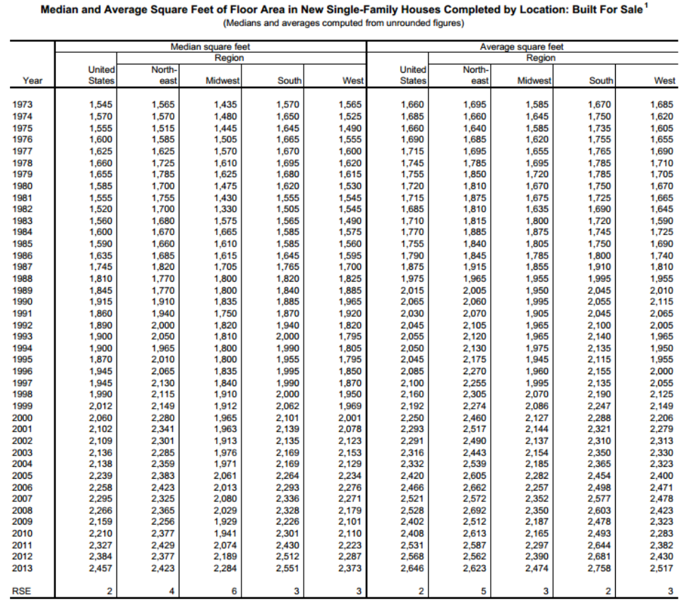
“Something about housing.  I’m sure you’ll find out all about it while you are eating.”

Mabel had set a nice lunch plate of panini bread, cheese and vegetables.  George was a tall man, a big boned man, prone to weight gain in retirement. Although George was fairly fit for his age, she worried about his health, particularly his heart, the male curse.  Mabel made sure that they both ate sensible, healthy meals.

Mabel took her lunch into the living room, leaving George alone in the kitchen.  He liked to check in on the stock market a few hours before the close to get a sense of the direction of the day’s action.  She would have chosen to keep all their savings in CDs and savings accounts but the interest rates were so low that living expenses would slowly erode their principle.

“We’ll put just 25% of our money in the market,” George had told her.  “I’ll watch it carefully and if anything like 2008 happens again, we can pull it out right away.  I’ll know what the signs are.”

George had studied a book on technical indicators which were supposed to help a person understand the direction of the market.  Despite her confidence in George’s ability and sensibility, Mabel still worried.  The stock market had always seemed to her like gambling.

At the kitchen table, George turned on the computer while he chewed his carrots and celery.  He had never been fond of vegetables but found that his likes and dislikes had mellowed with age.  He liked that Mabel cared.  The market helped distract him from the vegetables.  He paged through the daily calendar at Bloomberg, then checked out the headlines at Yahoo Finance. Existing home sales in August had fallen more than 5% from the previous August but that was a tough comparison because 2013 had been a pretty strong year.  Existing home sales were still above 5 million.

Before George had invested some of their savings in the stock market, he had bought several books on how to read financial statements but soon gave up when he realized that knowing the fundamentals of a company would not protect their savings in the case of another meltdown like the recent financial crisis.  Patient though she might be, Mabel would be extremely upset with him if he lost half of his investment in the market.

He then turned to the study of technical indicators which analyzed the behavior of other buyers and sellers in the stock market.  As an insurance adjuster, he had learned C programming back in the 1990s and found a charting program whose language was familiar to him.  As a former adjuster for the insurance of commercial buildings, he was used to making judgments based on a complex interplay of many factors.  He played with several indicators, found a few that seemed to be reliable, but got burned when the market melted down in the summer of 2011.  He got out quickly but not quickly enough for he had lost more than 10% of his investment in the market.  The market healed but at the time it seemed as though there might be a repeat of the 2008 crisis.  Had George and Mabel been younger, George could have just ridden out the storm.  Retirement had made him cautious and the 2011 downturn made George almost as leery of the market as Mabel.

Tuesday was a fine day in late September.  Mabel put her crochet down and made the two of them some soup, with fruit, crackers and cheese.  She took pride in the variety of food that she prepared.  When she walked out on the deck to call George in for lunch, a startled crow took to flight.  George was sitting on the edge of the deck where the crow had been.

“What are you doing, George?”
“I was teaching that little crow how to break open a peanut,” George replied. “I think they learn how to do stuff like that from their parents but I haven’t seen the flock in a few days and this guy was just wandering around the backyard looking for something to eat.  When I gave him a peanut, he didn’t seem to know what to do with it.  He’d pick it up in his beak, then drop it and stare at it.  He pecked at it a few times but that only made the peanut skitter away. “
George held up a branch.  “I carved a claw into the end of this branch and held down the peanut for him.”  George held up half a peanut shell.  “See, he got it figured out.  He flew off when the door opened but I’ll betcha he’ll be back.”
“Well, come on in then.  Lunch is ready.  The market is down again.  Something about housing again.”
“Hmmm,” George grunted and followed Mabel into the kitchen.  “Hmmm, that soup smells good.”
“A little beef vegetable that I doctored up a bit,” Mabel said with a smile.
George gave her a little hug. “I sure like your doctoring.”

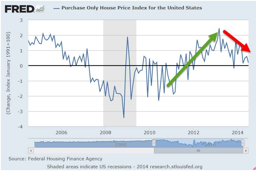
He sat down to eat, wondering what all the fuss in the market was.  Checking the Bloomberg Calendar, he saw that it was the House Price index from the Federal Housing Administration that had dampened spirits.  The monthly change was drifting down to zero, a sign of weakness.  Although housing prices were still rising, the rise was slowing down.

A disappointment, George thought, but not a catastrophe.  However, the market had been down for three days in a row.  He finished his lunch and went into the living room.  Mabel was reading a book.
“You know, Mabel, I think it’s just a short term thing.  The bankers from the developed countries met last week and they kinda put out a wake up call to the market.  I think there’s a bit more caution and common sense after that.”
“Well, as long as you’re watching it, dear.”
“You know, we did good this last year,” he reassured her.
“I just worry that it was too good.  We should have taken some of that out of the market and put it somewhere safe.”
 “Well, I’m keeping an eye on it,” he said.  “I checked CD rates last week and they are paying like 1% for a one year CD.  It just ain’t like it used to be. We just have to take some risk.”

They had a 3-year CD coming due in a month. He didn’t want to tell her that he was thinking about not rolling over the CD.  Maybe buy a bond fund.  She wouldn’t like that. For a time he had dabbled in some short to medium term trading but barely broke even.  He had lost sight of his original goal – to keep their savings safe while taking some risk with the money.  Fortunately, this insight had come to him toward the end of 2012.  The market had been mostly up since then, rewarding those who sat out the small downturns.

Late Wednesday morning, Mabel could hear George on the side of the house clearing brush or some such thing.  He said he was going to cut down an elm tree sapling that was growing near the house but when she went out to call him into lunch, he had cut everything but the elm sapling.

“I thought you were going to cut that down, dear.”
“Well, I was but the squirrels are using it to climb up to the old swamp cooler we have perched up there.  You remember the litter from early this spring?  Well, I think there’s another litter in there.  I haven’t seen any young ones but there’s a squirrel carrying twigs up that sapling to the cooler.  She’s even got a piece of one of my rags.  Must’ve fallen out of my pocket.”

Mabel looked up at the platform George had mounted to the side of the house years ago.  On top of the platform sat the old abandoned cooler.  George had meant to take it down and disassemble the platform but then the squirrels had used it as a nursery this winter and neither of them had been able to dismantle it while the little ones were scampering around in and out of the cooler.  Of course, George was supposed to take the cooler down during the summer but never got around to it.  Now she saw that he had tied a cord from the platform to the sapling to bend the sapling close to the platform, making it easier for the squirrel to get from the tree to the platform.

She shook her head and said “George Liscomb, I hope you don’t let that sapling get out of hand.  You know how elm trees are.  They grow faster than a puppy.”
“Well, the tree won’t grow much during the winter and I’ll cut it down in the spring.”
“Ok, well, come on it.  Lunch is ready.  I heard on the radio that the market is up a lot today.  Housing again.  Maybe you were right about it being short term.”
“Well, of course, I’m right,” he made a grand gesture.  “The squirrels will confirm that.”

His lunch plate held some broccoli spears and six, no more and no less, tater tots.  “I know you don’t particularly like broccoli so I thought a few tater tots might ease the pain,” Mabel said with a slightly sardonic smile.

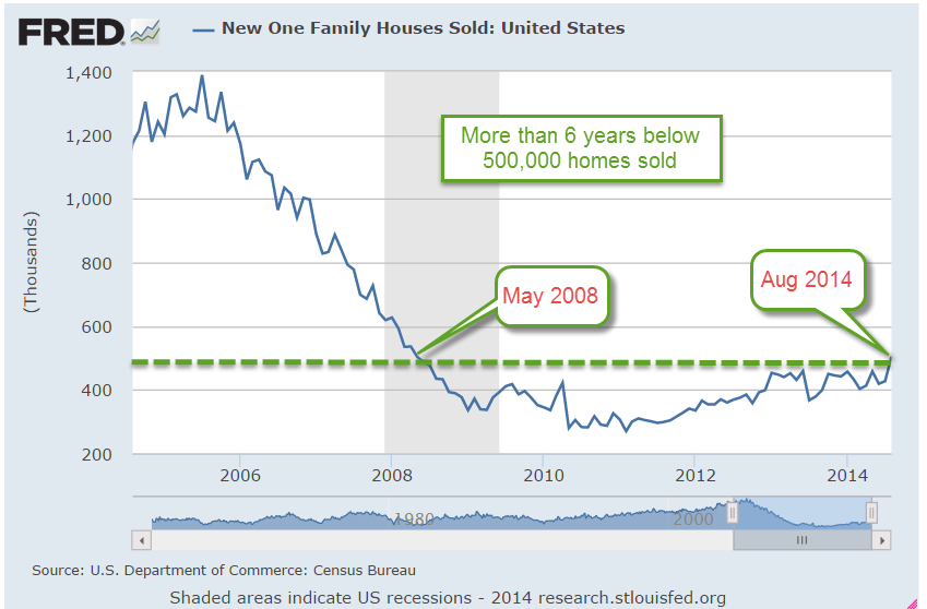
He laughed.  “I’m married to a kind prison guard.”  He sat down at the table, wondering what could have buoyed the market so much.  Housing yet again.  “Holy moly!” he called out to Mabel. He went into the living room to tell her the good news. “Finally, after more than six years, new homes are selling at a rate of more than half a million a year.  That’s what’s got the market dancing.”

On Thursday, she found George working on the stream that he had built in the rock garden.  A few feet from George a squirrel cautiously sipped water from the stream.  The squirrel saw her and scampered up the nearby fence.  “It’s remarkable how comfortable they are with you,” she told him.  “I try to move slowly when I’m working,” George replied. “They seem to be less anxious.”
“What are you doing today?” she asked.
“Got a leak somewhere.  I’ve lost about 15 gallons since last night.  Still haven’t found it.”
“Well, you’re not going to like what going on in the market.  It’s way down today and it’s not about housing.”

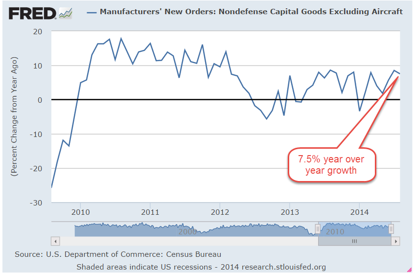
He followed her into the house and broke into a big grin when he saw what was for lunch. “Tuna fish!”  Mabel had dressed up her famous tuna fish salad with lettuce, tomatoes, some green onions and put it open faced on some toasted bread.  It was scrumptious.  Not so the market.  The SP500 was down about 1-1/2% on several news releases.  The whopper was that Durable Goods Orders were down 18% in August from the previous month.  But most of that drop was a decline in aircraft orders after a surge in those same orders in July.  Aircraft orders were notoriously volatile. Year-over-year gains in non-defense capital goods, the core reading, were up almost 8%.

The weekly report of new unemployment claims had risen slightly but was still below 300,000.  September’s advance reading of the services sector, the PMI Services Flash, was slightly less than the robust reading of August but still very strong.  So what was causing these overreactions to news releases?  The short term traders execute buy or sell orders within seconds of a news release.  Computer algorithms trade within nanoseconds of the release.  If new unemployment claims are up even by 1, the word “up” or “rise” or some variation will occur within the release.  Sell.  New home sales up?  Up is good for this report.  Buy.  Why would the short-termers be so active this week?  Because they are trading against each other.  The mid and long termers, the portfolio managers, will take the stage at the beginning of next week to adjust their positions at quarter end when funds report their allocations.

Late Friday morning, Mabel stood out on the back deck, her mouth open at the sight of George hunched down as he came out of the shed in the backyard.  Hundreds of wasps swarmed above him.  He knelt down and closed the doors to the shed and hurried to her on the deck.

“My God, George!  Are you all right?”
“Oh, yeah, no worries.  Anything on me?” he asked.
“No.”  There were just a few wasps visible outside the closed doors.  “What on earth?!”
“Well, they’ve really built themselves a city since I was in there last,” George explained.  He sat down on the deck.  The shed was where they kept old tax records and camping gear that they hadn’t used in quite a long time but hadn’t given away or sold – just in case they went camping again.  “I should have sprayed them earlier in the summer but it was such a small hive.  Those doors get sun most of the day so they like it in there.  They’re right above the doorway so they’re not bothering any of our stuff and I was able to stand up in the shed and they just left me alone.”
“I don’t care. What if I had gone out there to get something?!” she said angrily.
“Yeh, you’re right.  I’ll take care of them this weekend.  I was kinda waiting for the cold weather to do its job.”  He held up his hands a couple of feet apart from each other.  “That hive is like this, strung out along the studs that frame the doorway.”
“Why were you out there?” she asked.
“Well, I wanted to see if we still had the box that the TV came in a few years ago.”
“Didn’t you throw it out?” she asked.
“Well, I thought that in case we had trouble with the TV but then the box was behind a bunch of stuff and it was hard to get to and I guess I forgot,” he admitted.
“Well, come on it and eat your lunch.  The market is up again today, I heard them say.”

George settled down at the kitchen table.  A few salami slices, some macaroni salad, carrots, olives and crackers sat on the plate.  “Working man’s antipasto, hey?”
“There are some sardines in there, too” she said.
“I have the best wife and cook in the world.  Anthony Bourdain, move ovah!  Mah honey’s takin’ ovah!”
Mabel laughed.  “Now let me get back to my book.  Second to last chapter and I think the niece did it.  I haven’t trusted her since the first chapter.”

The 3rd estimate of 2nd quarter GDP had been revised up from 4.2% to 4.6%, helping to compensate for the weak first quarter.  Good stuff, thought George.  The U. of Michigan Consumer Sentiment Survey had risen in September to 84.6 from August’s 82.5.  Confident consumers buy stuff, a good sign.  Anything above 80 was welcome and more was better.  To round out the daily trifecta of news releases, corporate profits for the second quarter were revised upward.  The year over year gain without inventory and depreciation adjustments was 12.5%.  Not spectacular but solid.

Even with Friday’s triply good news, the market closed below what it opened at the previous day.  This was usually an indication that the short term downward trend in the market might have a little way to run.  Then he promised Mabel that he would get rid of the wasps this weekend, and yes, he would be careful.  Did she remember seeing the wasp spray that he bought earlier that summer?