Invisible Expectations

June 2, 2024

by Stephen Stofka

This week’s letter continues a topic from last week, our expectations of inflation. The high inflation of the 1970s prompted a lot of debate on this topic, and I will try to cover a portion of those ideas. Hypotheses regarding the formation of expectations influence monetary policy and the manner in which the Fed raises interest rates. Different policy approaches reach across the country into the pocketbooks of many Americans. They can mean the loss of many jobs or few jobs, or the viability of buying a home.

The University of Michigan conducts a monthly survey of consumer sentiment in a rotating sample among 500 participants. Respondents are asked to estimate the rate of inflation for the next twelve months (see here, p. 5). Inflation is a rise in the average price of all goods but in casual conversation, we often use the term loosely to refer to a rise in prices of the goods and services that have the most impact on our lives. Each of our estimates are biased but an average of many estimates should approximate a comprehensive survey of the prices of many goods. This BBC five-minute video explains this phenomenon known as The Wisdom of the Crowd when many people try to estimate the number of jelly beans in a mason jar.

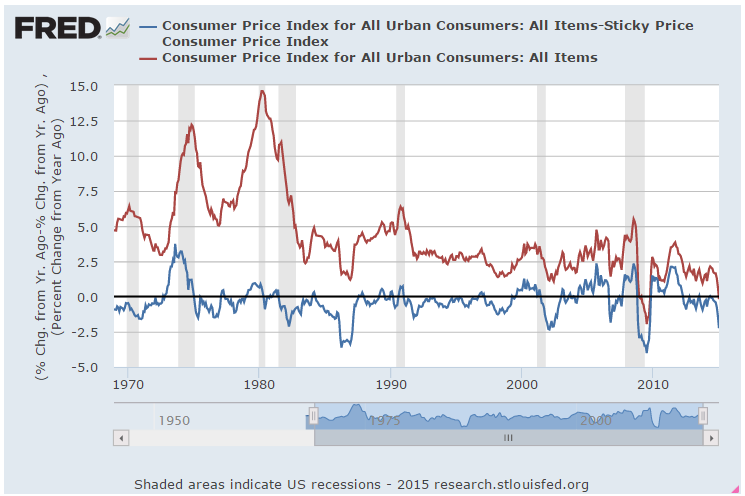
The blue line in the graph below is the headline CPI that tracks a basket of goods and excludes expenses like the employer portion of health care insurance. The Fed pays more attention to the PCEPI, the green line in the graph below. That methodology is based on actual expenditures in various sectors of the economy, including employer paid health insurance. Notice how closely the average estimates of inflation approximate this broad measure of price movement. In the April 2024 survey, expectations averaged 3.2%, a big decrease from over 5% in 2022 but a slight rise from 2.9% in March.

How do we form inflation expectations? There are two hypotheses, and they are distinguished by how errors occur in our expectations. Adaptive expectations was a predominant hypothesis until the 1970s. It holds that we revise our forecasts up when actual inflation is higher than we expected, and down when inflation data indicates that our forecast was too high (Blanchard, 2017). Imagine that we are offered a discount at the doctor’s office if we guess our weight within three pounds. We base our guess on a previous weight reading. If it is too low, we lose our discount so the next time we revise our guess higher. Under this hypothesis, our expectations are very much guided by past experience and our forecast errors are systemic. To tame high inflation, monetary policy must act like a shock that induces a recession and alters the expectations of investors and consumers.

In August 1979, during the Carter administration, Paul Volker assumed the position of Fed chair. In October, the Fed raised interest rates 1.5%, then lowered by a half-percent in November, then raised them again by a half-percent in December. In those three months, sales of new one-family homes (HSN1F) dropped 25%. A few months later, in the spring of 1980, came another interest rate shock of a 3.5% increase over two months and new one-family homes sank by 38%. They did not begin to recover until the spring of 1982. This cattle prod approach to taming expectations was influenced by the adaptive expectations hypothesis.

Statistical tests done in the early to mid-1970s showed that we paid much more attention to ongoing conditions than previously thought. This contradicted the notion that our expectations relied mostly on past experience. Two economists, Robert Lucas and Thomas Sargent presented a rational expectations hypothesis claiming that we form the best inflation forecast we can with the information available to us. Rational does not mean perfect. Errors in our forecasts are random and arise from unseen shocks (Humphrey, 1985). The critique against this hypothesis was that people were too naïve or uninformed to form rational expectations. Information frictions blurred the distinction between rational and non-rational (Angeletos et al, 2021).

 Over the past several decades, the rational expectations hypothesis has guided policymaking at the Fed. If the Fed presents a convincing policy commitment to steer inflation toward a particular target, investors will change their behavior in accordance with their belief in the Fed’s commitment. Economist Roger Farmer (2010) has called them self-fulfilling beliefs and devotes a section of his book to rational expectations. Under this regime, the Fed uses steady, incremental rate increases and consistent policy statements to “corral” expectations like a trained sheepdog persistently badgering a flock of sheep to guide them into a holding area. By guiding expectations, monetary policy can tame high inflation without necessarily producing a recession. This has been dubbed a soft landing.

In the spring of 2022, the Fed under Chairman Jerome Powell raised rates a half percent a month, a steady rate to let everyone know that the Fed was serious. From the spring of 2022, the number of new one-family homes did not fall. That was the rational expectations hypothesis at work. The Federal Reserve as sheepdog. As with any comparison, there are a number of other factors. My point here is that ideas about people’s motivations and behavior make a concrete difference in the lives of ordinary people.

We respond to high inflation with behavior that can exacerbate inflation. Next week I will look at several scenarios that illustrate why the Fed is concerned about managing consumer and investor expectations.

///////////////////

Photo by Hassaan Here on Unsplash

Keywords: housing, interest rates, monetary policy, adaptive expectations, rational expectations, inflation

Angeletos, G.-M., Huo, Z., & Sastry, K. A. (2021). Imperfect macroeconomic expectations: Evidence and theory. NBER Macroeconomics Annual, 35, 1–86. https://doi.org/10.1086/712313

Blanchard, O. (2017). Macroeconomics (Seventh ed.). Boston, MA: Pearson Education. p. 337. This is an intermediate economics textbook.

Farmer, R. E. A. (2010). How the economy works: Confidence, crashes and self-fulfilling prophecies. Oxford University Press. This book contains succinct descriptions of various economic theories that have influenced policy and is aimed toward the general reader.

Humphrey, Thomas M., The Early History of the Phillips Curve (1985). Economic Review, vol. 71, no. 5, September/October 1985, pp. 17-24, Available at SSRN: https://ssrn.com/abstract=2118883

Price Waves

May 19, 2024

by Stephen Stofka

This week’s letter is about our perception of inflation and the uncomfortable feelings we experience at higher-than-expected changes in prices. We notice price changes relative to the goods and services we experience and purchase in our daily lives. If the water is rising under our boat, we reason that the water is rising under all boats. We may have a good understanding of local conditions but a less accurate picture of underlying trends in a national economy. Economists understand the term on a macro level, when most people experience rising prices in the bundle of goods they buy. Inflation is a rise in the average of all prices for consumer purchases and often reflects price changes throughout the supply chain. To gather this information, the Bureau of Labor Statistics and the Census Bureau interview households and businesses from around the country each month. The monthly report on inflation may confirm our intuitive sense of changing prices or it may challenge our own appraisal. With all those resources and data, why do economists argue over the causes of inflation? In either case, we experience high inflation as a loss of purchasing power, and that sense of loss is magnified by the particular attention we pay to losses.

The Federal Reserve and most central banks around the world try to keep inflation at about 2% per year. That rate is thought to compensate for measurement error and a rise in the quality of goods. Our tendency to ignore small changes is evident in other areas of our lives. The 410-mile journey west on I-70 through Kansas is almost flat, yet in that span there is gain in elevation of 3258 feet (calculations in notes). Expectations play a key role in the decisions that people and companies make. Central bankers want small changes in the average price to play a negligible role in those decisions. Claude Shannon wrote that if what happens tomorrow is what happened today, then there is no new information. Our attention is piqued by news, or new information, so that we tend to pay attention to deviations from that average. The average becomes our environment. Statisticians recapture this human tendency when they standardize or normalize an average by setting it to 0, called a z-score.

We integrate quality improvements into our expectations so that gradual improvements are little noticed. In 35 years a 2% annual improvement in the quality of a product or service will result in a doubling of its quality. The reliability, safety, efficiency and performance of cars today are vastly superior to the cars in the 1970s. In 2020, the price of a new car was about 50% higher than in 1980, an annual price increase of less than 2%. I will leave the series identifier in the notes.

The quality of cars has increased far more than the increase in price. During that time, control of many systems within a car transitioned from mechanical control to precise electronic control, improving fuel efficiency. The quality of tires improved, reducing the number of flats that forces a driver to the side of the road. Air conditioners perform better and do not need to be recharged every few years because the seals leak. In 1980, the design of a car transferred too much of the impact of a crash to the driver. Today, a car is designed to absorb and distribute those physical forces. Seat belts protect the passengers from being thrown about during an accident, while front and side airbags cushion a violent change in direction. Quality has improved by at least twice the 50% increase in price.

During the high inflation of the 1970s, the real weekly earnings of wage and salary workers (LES1252881600) fell, as shown in the chart below. The term real means inflation-adjusted. In an age when families paid their monthly bills by check or money order, rapidly increasing costs sometimes meant that there was not enough money to pay all the bills. Although the recent surge in inflation has invited comparisons with the 1970s, workers’ earnings have outpaced inflation in this past decade and shown real gains.

If wage gains are rising faster than prices, why do consumer sentiment surveys not reflect this economic reality? Economist Paul Krugman had a short and helpful op-ed on the sentiment gap in recent surveys. Consumer purchasing power has increased since the pandemic, but consumer sentiment has declined by an amount comparable to the Great Recession in 2007-2009 when purchasing power decreased. He shows evidence from other surveys that one’s political party affiliation is strongly correlated with changes in consumer sentiment. People who usually vote Republican are optimistic about the economy when a Republican is President. Democrats express positive feelings when a Democrat is in the White House.

Political alliances are easily exploited via social media, whose use has skyrocketed since the Great Recession began at the end of 2007. Negative news and negative views proliferate on social media because we have a tendency to pay more attention to bad news. In the newspaper business, the rule was “If it bleeds, it leads.” Taking advantage of this human tendency, anonymous accounts on social media post total fabrications in order to get views. Higher views earn more revenue from ad placement, turning bad news into good news for the poster. News that gives the reader a sense of uplift or empowerment can be treated as “Pollyannish.” What other factors might account for the discrepancy between sentiment and reality? One aspect might be a rising standard of living.

Just as the quality of cars has increased, so has our standard of living in general. Families today are used to a higher standard with more conveniences than was typical fifty years ago. More conveniences equals more bills. These include monthly cell phone costs, TV and cable subscriptions, and higher electrical costs to run all the new appliances, computers and entertainment devices we have today. Some homeowners may experience fees for trash pickup or parking fees that were not typical in decades past.

Higher prices feel like a loss to us, and we pay attention to losses more than we do the wage gains. Economists Daniel Kahneman and Amos Tversky (1977) invented behavioral economics when they presented compelling evidence that our decisions are not always rational, that we weigh gains and losses on different scales. This challenged the conventional view that people’s choices were fundamentally rational, that bad decisions or poor choices were due to errors in judgment or a lack of information. Kahneman and Tversky asserted that irrational decisions were systematic rather than random error. Our tendency to measure gains and losses with different yardsticks can help explain why we become accustomed to improvements in our lives so that they escape our attention. Losses challenge our survival more than wins so we give losses our greater attention.

We survive by reacting promptly to threats. Children are taught to curb this natural impulse, to use their words, not their fists when responding to the behavior of other young children. We do not hit the butcher in the grocery store because the price of a steak has gone up 20%, but we might feel a bit of anger or resentment toward some nameless cause of the higher price. Even though inflation is part of our economic environment, it is not like the weather, we reason. Human decisions cause inflation so someone is responsible. However, the cause is more likely to be a composite of human behavior, of natural biases in how we process and react to information. That would make each episode of high inflation a unique blend of circumstance and policy decisions unlikely to be repeated in the future.

Economists, ever on a quest to find the Holy Grail, to understand the underlying process of high inflation, cannot admit the singularity of each episode. Next week, I will explore some of the factors that contribute to episodes of high inflation. Until then, watch Monty Python and the Holy Grail.

//////////////

Photo by Tadeu Jnr on Unsplash

Keywords: monetary policy, Prospect Theory, inflation

Bernstein, P. L. (1998). Against the Gods. John Wiley & Sons. In Chapter 16, Bernstein explores the ideas in Prospect Theory proposed by Kahneman and Tversky.

Kahneman, D., & Tversky, A. (1977). Prospect Theory. an Analysis of Decision Making under Risk. https://doi.org/10.21236/ada045771.

The index on new car prices is https://fred.stlouisfed.org/series/CUUR0000SETA01 The series identifier for the used car price index is CUSR0000SETA02.

Journey through Kansas: Kansas City on the eastern border is 909′ in elevation. Burlington, CO, at the western border of Kansas is 4167′, a rise of 3258′, or 0.617 miles. Dividing Hays, KS on the west side of Kansas is 2018′, a rise of 1000 feet. The state is 410 miles wide so the 1000′ gain in elevation is only .05% per mile. The 3000 gain in elevation is .15% per mile, a grade that feels flat to us.

Cycle of  Expectations

January 28, 2024

by Stephen Stofka

This week’s letter is about the decisions people make in connection with their compensation. Guided by the strength of the job market and expectations of inflation, employees seek higher compensation by switching jobs or by wage and benefit demands. Like fish in the sea, these individual decisions form schools that follow and shape the currents of economic growth and inflation.

There are two main components to employee compensation. The first category includes wages or salary, some of which is reduced by income and FICA taxes. The amount left over is called disposable income. The second component of compensation is loosely categorized as benefits that are already dedicated to a single purpose and are non-disposable. These include paid time off, pension plan contributions and health care. They also include government mandated taxes that the employer pays for the employee. These include workers’ compensation, unemployment insurance and the employer’s half of FICA taxes. Except for paid time off, employees do not pay income taxes on benefits.

As I noted last week, the Bureau of Labor Statistics calculates an Employment Cost Index (ECI) that includes both wages and benefits. This composite can give us different insights than tracking the growth of wages alone. Comparing the ratio of the wages portion to the total index allows us to spot trends when wages grow more than benefits or benefits grow faster than wages. I’ll call this the Wage Ratio.

In the chart below, we can see three distinct periods: 2001 through 2007, 2008 through 2015, and 2016 through 2023. In the first and third periods, wages grew faster than benefits but their growth patterns are distinct. In the first period growth was coming into balance with benefit growth. In the third period, wage growth was accelerating. In both periods there was a strong correlation between the wage ratio and an inflation measure that the Fed uses called PCE inflation (see notes).

When inflation is low, employees may desire more of their compensation in benefits. Most of these are tax-free so employees get more “bang” for each dollar of benefit. In the second period, there was a rebalancing of wages and benefits. As the nation recovered from the housing and financial crisis, low inflation reduced the pressure to seek higher wages. During the last year of Obama’s second term in 2016, that inflation rate began to rise from near zero to 2%. The Fed raised its key interest slightly above zero, happy to finally see inflation nearing the 2% target rate that the Fed considers healthy for moderate growth.

The Fed also has a target for its key interest rate that is 2% or above. For eight years it had kept that interest rate near zero to help the economy recover after the financial crisis. The Fed knows that such a low rate has two disadvantages. It gives the Fed less room to respond to economic crises because they cannot adjust rates lower than the Zero Lower Bound (ZLB). Secondly, sustained near-zero rates lead to high asset valuations, or bubbles, which are disruptive when they pop. The housing crisis was a recent example of this.

During the first three years of the Trump presidency, inflation leveled out near that 2% target rate as the Fed continued to raise rates in small increments, finally ending near 2.5%. In 2018, Trump went on a tirade against the Fed, accusing it of sabotaging his Presidency. Low interest rates had fueled an annual rise in housing prices from 5% at the end of Obama’s term to 6.4% in the first quarter of 2018. Trump was not the first President who wanted a subservient Fed willing to enact policy that enhanced the Presidential political agenda. Because a President wins a general election, they may convince themselves that their desires reflect the general will. They do not. Congress gave the Fed a twin mandate of full employment and stable prices to separate Fed policy from Presidential control. It did so after several episodes where Fed policy served the desires of the President rather than the public welfare.

In 1977, Biden was in the Senate when Congress enacted the legislation that gave the Fed a twin mandate. Unlike Trump, Biden has not pounded his chest like a belligerent gorilla as the Fed raised rates by five percentage points within a year. The results of the Republican primaries in Iowa and New Hampshire make it likely that this year’s election will be a repeat contest between Biden and Trump. The Fed has hinted that they might lower rates this year if inflation indicators remain stable and the unemployment rate remains low. That would be the proper response and in accordance with the Fed’s mandate.

Should the Fed lower rates even a small amount, Trump will certainly complain that the Fed is helping Biden win re-election. He will protest that “the system” is opposed to him and his MAGA supporters. If Republicans can gain control of both houses of Congress and the Presidency this November, Trump will likely pressure McConnell to change the cloture rule so that Senate Republicans will need only a majority to pass a bill making the Fed an agency subject to Trump’s control. In 2022, seven Republican Senators introduced a bill to condense the number of Federal Reserve banks and make their presidents subject to Senate approval. Should the Fed lose its independence from political control, we can expect the high inflation that has afflicted Venezuela and Argentina, countries where a political leader has used monetary policy to win political support. Workers will demand higher wages to cope with rising prices and those demands will help fuel the inflationary cycle. We actualize our expectations.

/////////////////

Photo by Erlend Ekseth on Unsplash

Keywords: inflation, wage growth, housing prices, Fed policy, monetary policy

Correlation: In the eight year period from 2001thru 2008 when wage growth was high but declining, the correlation between inflation and wages was -.63. From 2016 through 2023, as the wage ratio was rising, the correlation was .85.

Home Prices and Monetary Policy

July 30, 2023

by Stephen Stofka

This week’s letter is a proposal for an alternative measure to guide the Fed’s monetary policy. In 1978, Congress passed the Full Employment and Balanced Growth Act which gave the Fed a dual mandate – giving equal importance to price stability and full employment. The Canadian central bank has a hierarchical mandate with price stability as a priority. As with most Congressional mandates, the legislation left it up to the agency, the Fed, to determine what price stability and full employment meant. The Fed eventually settled on a 2% inflation target. Full employment varies between 95-97% and is hinged on inflation.

For its measure of inflation, the Fed relies on the Bureau of Labor Statistics (BLS) who conducts monthly surveys of consumer expenditures.  The BLS compiles a CPI based on the its price surveys of hundreds of items. The Fed prefers an alternative measure based on the Consumer Expenditure Survey, but the weakness in both measures is the complexity of the methodology and the inherent inaccuracy of important data points.

According to the BLS, housing costs account for more than a third of the CPI calculation. Twenty-five percent of the CPI is based on an estimate of the imputed rental income that homeowners receive from their home. This estimate is based on a homeowner’s response to the following question:   “If someone were to rent your home today, how much do you think it would rent for monthly, unfurnished and without utilities?” How many owners pay close attention to the rental prices in their area?  The BLS also surveys rental prices but tenants have six to 12 month leases so these rental estimates are lagging data points. The BLS tries to reconcile its survey of rents with homeowners’ estimates of rents using what it admits is a complex adjustment algorithm. 

The BLS regards the purchase of a home as an investment, not an expenditure so it must make these convoluted estimates of housing expense. There is a simpler way. Buyers and sellers capitalize income and expense flows into the price of an asset like a house. The annual growth in home prices would be a more reliable and less complex measure of inflation. Federal agencies already publish monthly price indexes based on mortgage data, not homeowner estimates and complex methodology. An all-transactions index includes refinancing as well as purchases. Bank loan officers have a vested interest in monitoring local real estate prices so their knowledge is an input to the calculation of a home’s value when an owner refinances.

The Federal Housing Finance Agency (FHFA) publishes the All-Transactions House Price Index based on the millions of mortgages that Fannie Mae and Freddie Mac underwrite. From 1990 – 2020, home prices rose by an average of 3.5% per year. A purchase only index that does not include refinances rose almost 3.9% during that period. As an aside, disposable personal income rose an average of 4.6% during that period.

The Fed does not need authorization from the Congress to adopt an alternative measure of inflation to guide monetary policy. As its strategy for price stability, the Fed could set a benchmark of 4% – 5% home price growth, near the 30 year average. If house prices are rising faster than that benchmark, monetary policy is too accommodating and the Fed should raise rates. Since the onset of the pandemic, home prices have risen 11% per year, three times the 40 year average. This same growth marked the peak of the housing boom in 2005-2006 before the financial crisis. The Fed did not begin raising interest rates until the spring of 2022. Had it used a home price index, it would have reacted sooner.

The annual growth in home prices first rose above 4% in the second quarter of 2013. The Fed kept interest rates at near zero until 2016, helping to fuel a boom in both the stock market and housing market. Since 2013, house prices have stayed above 4% annual growth, helping to fuel a surge in homelessness. Let’s look at several earlier periods when using home prices as a target would have indicated a different policy to monetary policymakers at the Fed.

In 1997, the annual growth of home prices rose above 4% and remained elevated until the beginning of 2007 when the housing boom began to unravel. In 2001, home prices had risen almost 8% in the past four quarters but the Fed began lowering its benchmark Federal Funds rate from 5.5% to just 1% at the start of 2004. The Fed was responding to increasing unemployment and a short recession following the dot-com bust. Near the end of that recession came 9-11. By lowering rates the Fed was pushing asset capital that had left the stock market into the housing market where investors took advantage of the spread between low mortgage rates and high home price growth.

In 2004, home price growth was over 8% and accelerating. Had the Fed been targeting home prices, it would have acted sooner. However, the Fed waited until the general price level began rising above its target of 2%. In the 2004-2006 period, the Fed raised rates by 4%, but it was too late to tame the growing bubble in the housing market. In 2005, home prices grew by 12% but began responding to rising interest rates. By the first quarter of 2007, home price growth had declined to just 3.3%.

The Fed models itself as an independent agency crafting a monetary policy that is less subject to political whims. However, the variance in their policy reactions indicates that the Fed is subject to the same faults as fiscal policy. If the Congress is crippled, then the Fed feels a greater pressure to react and is helping to fuel the boom and bust in asset markets. Let’s turn to the issue of full employment.

The condition of the labor market is guided by two surveys. The employer survey measures the change in employment but does not capture a lot of self-employment. The household survey captures demographic trends in employment and measures the unemployment rate. The BLS makes a number of adjustments to reconcile the two series. The collection of large datasets and the complex adjustments needed to reconcile separate surveys naturally introduces error.

The labor market has experienced large structural changes in the past several decades. Despite that, construction employment remains about 4.5 – 5.5% of all employment so it is a descriptive sample of the condition of the overall market. Declines in construction employment coincide with or precede a rise in the unemployment rate. In the past 70 years, the construction market has averaged 1.5% annual growth. During the historic baby boom years of the 1950s and 1960s, the growth rate averaged 2%. The Fed might set a target window of 1.5% – 2.5% annual growth in construction employment. Anything below that would warrant accommodative monetary policy. Anything above that would indicate monetary tightening. In 1999, the growth rate was 7%, confirming the home price indicator and strongly suggesting that fiscal or monetary policy was promoting an unsustainable housing sector boom.  

If the Fed had adopted these targets, what would be its current policy? The FHFA releases their home price data quarterly. The growth in home prices has declined in the past year but was still 8.1% in the first quarter of 2023. However, the S&P National Home Price index tracks the FHFA index closely and it indicates a slight decline in the past 4 quarters. Growth in construction employment has leveled at 2.5%, within the Fed’s hypothetical target range. The combination of these two indicators would signal a pause in interest rate hikes. This week, the Fed continued to compound its policy mistakes and raised interest rates another ¼ percent.  

////////////

Photo by Rowan Heuvel on Unsplash

Slow Growth

April 21, 2019

by Steve Stofka

Happy Passover and Happy Easter. Now that tax day is past, let’s raise our heads and look at long-term growth trends of real, or inflation-adjusted, GDP. For the past seventy years real GDP has averaged about 3% annual growth. In the chart below, I’ve charted the annual percent change in a ten-year average of GDP (GDP10, I’ll call it). As you can see on the right side of the graph, growth has been below average for the past decade.

In 2008, growth in the GDP10 crossed below 3%. Was this due to the Financial Crisis (GFC) and the housing bust? No. The GFC barely figured into the computation of the ten-year average. The housing market had been running hot and heavy for four to five years, but this longer-term view now puts the housing boom in a new perspective: it was like lipstick on an ugly pig. Without the housing boom, the economy had been faltering at below average growth since the 1990s tech boom.

The stock market responds to trends – the past – of past output (GDP) and the estimation of future output. Let’s add a series of SP500 prices adjusted to 2012 dollars (Note #1).

For three decades, from the late 1950s to the mid-1980s, the real prices of the SP500 had no net change. The go-go years of the 1960s raised nominal, but not real, prices. Investors shied away from stocks, as high inflation in the 1970s hobbled the ability of companies to make real profit growth that rewarded an investor’s risk exposure. From the 2nd quarter of 1973 to the 2nd quarter of 1975, real private domestic investment lost 27% (Note #2). In less than a decade, investment fell again by a crushing 21% in the years 1979 through 1982.

In the mid-1980s, investors grew more confident that the Federal Reserve understood and could control inflation and interest rates. During the next decade, investors bid up real stock prices until they doubled. In 1996, then Fed chairman Alan Greenspan noted an “irrational exuberance” in stock prices (Note #3). The “land rush” of the dot-com boom was on and, within the next five years, prices would get a lot more exuberant.

The exuberance was well deserved. With the Fed’s steady hand on the tiller of money policy, the ten-year average of GDP growth rose steadily above its century-long average of 3%. A new age of prosperity had begun. In the 1920s, investment dollars flowed into the new radio and advertising industries. In the 1990s, money flowed into the internet industry. Construction workers quit their jobs to day trade stocks. Anything less than 25% revenue growth was the “old” economy. The fledgling Amazon was born in this age and has matured into the powerhouse of many an internet investor’s dream. Thousands of other companies flamed out. Billions of investment dollars were burned.

The peak of growth in the ten-year average of GDP output came in the 1st quarter of 2001. By that time, stock prices had already begun to ease. In the next two years, real stock prices fell almost 50%, but investment fell only 12% because it was shifting to another boom in residential housing. As new homes were built and house prices rose in the 2000s, long-term output growth began to climb again.

From the first quarter of 2006 to the 3rd quarter of 2009, investment fell by a third, the greatest loss of the post-war period. In the first quarter of 2008, growth in the GDP10 fell below 3%. In mid-2009, it fell below 2%. Ten years later, it is still below 2%.

The Federal Reserve has had difficulty hitting its target of 2% inflation with the limited tools of monetary policy. There simply isn’t enough long-term growth to put upward pressure on prices.  Despite the low growth, real stock prices are up 150% since the 2009 lows.  A prudent investor might ask – based on what?

The supply side believers in the Trump administration and Republican Party thought that tax cuts would spur growth. In the first term of the Obama administration, believers in Keynesian counter-cyclical stimulus thought government spending would kick growth into gear. Faced with continued slow growth, each side has doubled down on their position. We need more tax cuts and less regulation, say Republicans. No, we need more infrastructure spending, Democrats counter. Neither side will give up and, in a divided Congress, there is little likelihood of forging a compromise in the next two years. The stock market may be waiting for the cavalry to ride to the rescue but there is no sign of dust on the horizon.

Economists are just as dug in their ideological foxholes. The Phillips curve, the correlation between employment and inflation, has broken down. The correlation between the money supply and inflation has also broken down. High employment but slow output growth and low inflation. Larry Summers has called it secular stagnation, a nice label with only a vague understanding of the underlying mechanism. If an economist tells you they know what’s going on, shake their hand, congratulate them and move to the other side of the room. Economists are still arguing over the underlying causes of the stagflation of the 1970s.

A year ago, I suggested a cautious stance for older investors if they needed to tap their assets for income in the next five years. The Shiller CAPE ratio, a long-term evaluation of stock prices, is at the same level as 1929. At current prices in a low growth environment, stock returns may  struggle to average more than 5-6% annually over the next five years.

//////////////////////

Notes:

  1. Adjusted for inflation by the Federal Reserve’s preferred method, the Personal Consumption Expenditures Price Index (FRED series PCEPI). Prices do not include dividends
  2. Real Gross Private Domestic Investment – FRED Series GPDIC1.
  3. A video of the 1996 “irrational exuberance” speech

The Start of the Beginning

April 7, 2019

by Steve Stofka

In 1971 former President Nixon announced that the U.S. was abandoning the gold standard of fixed exchange that had existed for almost thirty years. Within a short time, other leading nations followed suit. Each nation’s currency simply traded against each other on a global currency, or FX, market.

Since oil was priced in dollars and the world ran on oil, the U.S. dollar became the world’s reserve currency. Each second of every day, millions of US dollars are traded on the international FX markets. The demand for US dollars is strong because we are a productive economy. The euro, yen and British pound are secondary currency benchmarks.

When the U.S. wants to borrow money from the rest of the world, the U.S. Treasury sells notes and bills collectively called “Treasuries” to large domestic and foreign banks who “park” them in their savings accounts at the Federal Reserve (Fed), the U.S. central bank (Note #1). The phrase “printing money” refers to a process where the Federal Reserve, an independent branch of the Federal Government, buys Treasury debt on the secondary market. It may surprise many to learn that the Fed owns the same percentage of U.S. debt as it did in 1980. The debt in real dollars has grown seven times, but the percentage held by the Fed is the same. That is a powerful testament to the global hunger for U.S. debt. Here’s the chart from the Fed’s FRED database.

FedResHoldTreasPctDebt

In 1835, President Andrew Jackson paid off the Federal debt, the one and only time the debt has been erased. It left the country’s banking system in such a weak state that subsequent events caused a panic and recession that lasted for almost a decade (Note #2). Government debt is the private economy’s asset. Paying down that debt reduces those assets.

About a third of the debt of the U.S. is traded around the world like gold. It is better than gold because it pays interest and there are no storage costs. Foreign businesses who borrow in dollars must be careful, however. They suffer when their local currency depreciates against the dollar. They must earn even greater profits to convert their local currency to dollars to make payments on those dollar-denominated loans.

Each auction of Treasury debt is oversubscribed. There isn’t enough debt to meet demand. In a world of uncertainty, the U.S. government has a long history of respect for its monetary obligations. As the reserve currency of the world, the U.S. government can spend at will. Even if there were no longer a line of domestic and foreign buyers for Treasuries, the Federal Reserve could “purchase” the Treasuries, i.e. print money. Let’s look at the difference between borrowing from the private sector and printing money.

When the private sector buys Treasuries, it is effectively trading in old capital that cannot be put to more productive use. That old capital represents the exchange of real goods at some time in the past. In contrast, when the government spends by buying its own debt, i.e. printing money, it is using up the current production of the private sector. This puts upward pressure on prices. Let’s look at a recent example.

Quantitative Easing (QE) was a Fed euphemism for printing money. During the three phases of QE that began in 2009, the Fed bought Treasury debt. That was an inflationary policy that countered price deflation as a result of the Financial Crisis. In August 2009, inflation sank as low as -.8% (Note #3). It was even worse, but inflation measures do not include the dividend yield on money. To many households, inflation felt like -2% (Note #4). The Fed’s first round of QE did provide a jolt that helped drive prices up by 3% and out of the deflationary zone.

During the five years of QE programs, the Fed continued to fight itself. The QE programs pushed prices upwards. Near zero interest rates produced a deflationary counterbalance to the inflationary pressures of printing money. Because inflation measures do not include the yield on money, the Fed could not read the true change in the prices of real goods in the private sector. The economy continues to fall below the Fed’s goal of 2% inflation. There are still too many idle resources.

Leading proponents of Modern Monetary Theory (MMT) remind people that yes, the U.S. can spend at will, but that it must base its borrowing on policy rules to avoid inflation. A key component of MMT is a Job Guarantee (JG) program ensuring employment to anyone who wants a job. A JG program may remind some of the WPA work programs during the Great Depression. Visitors to popular tourist attractions, from Yellowstone Park in Wyoming to Carlsbad Caverns in New Mexico, use facilities built by WPA work crews. Today’s JG program would be quite different. It would be locally administered and targeted toward smaller public works so that the program was flexible.

The U.S. government has borrowed freely to go to war and has never paid that debt back. Proponents of MMT recommend that the U.S. do the same during those times when the private economy cannot support full employment. That policy goal was given to the Fed in the 1970s, but it has never been able to meet the task of full employment through crude monetary tools. With an active program of full employment, the Fed would be left with only one goal – guarding against inflation.

There are two approaches to inflation control: monetary and fiscal. Monetary policy is controlled by the Fed and includes the setting of interest rates. If the Fed’s mandate was reduced to fighting inflation, it could more readily adopt the Taylor rule to set interest rates (Note #4).

Fiscal policy is controlled by Congress. Because taxation drains spending power from the economy, it has a powerful control on inflation. However, changes in tax policy are difficult to implement because taxes arouse passions. We are familiar with the arguments because they are repeated so often. Everyone should pay their “fair share,” whatever that is. Some want a flat tax like a head tax that cities like Denver have enacted. Others want a flat tax rate like some states tax incomes. Others want even more progressive income taxes so that the rich pay more and the middle class pay less. Some claim that income taxes are a government invasion of private property rights.

Because tax changes are difficult to enact, Congress would be slow to respond to changes in inflation. The Fed’s control of interest rates is the more responsive instrument. The JG program would provide stability to the economy and reduce the need for corrective monetary action by the Fed. The program would help uplift those in marginal communities and provide much needed assistance to cities and towns which had to delay public works projects and infrastructure repair because of the Financial Crisis. As sidewalks and streets get fixed and graffiti cleaned, those who live in those areas will take more pride in their town, in their communities, in their families and themselves. This makes not just good economic sense but good spiritual sense. We can start small, but we must start.

////////////////////////
Notes:

1. Twenty to twenty-five times each month, the Treasury auctions U.S. government debt. Many refer to the various forms of bills and notes as “treasuries.” A page on the debt
2. The Panic of 1837
3. The Federal Reserve’s preferred measure of inflation is the Personal Consumption Expenditure Index, PCEPI series.
4. The annual change in the 10-Year Constant Maturity Treasury fell below -1% at the start of the recession in December 2007 and remained below -1% until July 2009. FRED series DGS10. John Maynard Keynes had recommended the inclusion of money’s yield in any index of consumer demand. In his seminal work Foundations of Economic Analysis (1947), economist Paul Samuelson discussed the issue but discarded it (p. 164-5). Later economists did the same.
5. The Taylor rule utility at the Atlanta Federal Reserve.


Hunt For Inflation

July 15, 2018

by Steve Stofka

Saddle up your horses, readers, because we are going on the Hunt for Inflation. I promise you’ll be home for afternoon tea. During this recovery, Inflation has been a wily fox, a real dodger. It has not behaved according to a model of fox behavior. Has Inflation evolved a consciousness?

Inflation often behaves quite predictably. The central bank lowers interest rates and pumps money into the economy. Too much money and credit chasing too few goods and Inflation begins running amuck. Tally-ho! Unleash the bloodhounds! The central bank raises interest rates which curbs the lending enthusiasm of its member banks through monetary policy. Inflation is caught, or tamed; the bloodhounds get bored and take a nap.

Not this time. Every time we think we see the tail of Inflation wagging, it turns out to be an illusion. Knowing that Inflation must be out there, the central bank has cautiously bumped up interest rates in the past two years. Every few months another bump, as though unleashing one more bloodhound ready to pounce as soon as Inflation shows itself.

Yes, Inflation has evolved a consciousness – the composite actions of the players in the Hunt. These players come in three varieties. One variety is the private sector – you and me and the business down the street. The second variety is the federal government and its authorized money agent, the Federal Reserve, the country’s central bank. Finally, there is a player who is a hybrid of the two – banks. They are private but have super powers conferred on them by the federal government. The private sector is the economic engine. The federal government and banks have inputs, drains and reservoirs that control the running of the economy.

The three money inputs into the constrained (see end) economy are 1) Federal spending, 2) Credit growth, and 3) net exports. In the graph below, the blue line includes 1, 2, and 3. The red line includes only 1. The graph shows the dramatic collapse of credit growth in this country. Federal spending accounted for all the new money flows into the economy.

CreditNXFedSpendvsFedSpend

Before the financial crisis, money flows into the economy were just over 30% of GDP. In less than a year, those inputs collapsed by almost 25%.

CreditGrowthFedSpendPctGDP

When inflation is lower than target, as it has been for the past decade, too much money flow is being drained out for the amount that is flowing in. In the case of too high or out of control inflation, as in the case of Venezuela, the opposite is true. Too much is being pumped in and not enough is being drained out. That’s the short story that gets you back to the lodge in time for a cup-pa or a pint. Next week – the inputs, drains and reservoirs of the economy.

////////////////////////////

  1. Constrained – the private economy, state and local governments who cannot create new credit.
  2. Net exports are the sum of imports (minus) and exports (plus).

Intervention

August 27, 2017

Pew Research surveyed four generations of Americans, from the oldest Americans who are part of the Silent Generation, those who grew up during the Great Depression, to the Millennials, those born between the years 1983 – 2002. Pew asked the respondents to list ten events (not their own) or trends that happened during their lifetime that had the most influence on the country. 9-11 was at the top of the list for all four generations. Obama’s election, the tech revolution and the Iraq/Afghanistan war were the other events common on each list. Some differences among the generations were understandable. Some were a surprise to me. The Great Recession/Financial Crisis of 2008 was only on the Millennials list. Many in this generation were in the early stages of their careers when the recession began. Here is a link to the survey results. Perhaps you would like to make your own list. Keep in mind that the events must have happened during your lifetime.

I don’t think that the Boomer generation understands the long-term impact of the Great Recession. In another decade, many will discover how vulnerable the financial crisis left all of us, not just the Millennials. As we’ll see below, the crisis may be over but the response to the crisis is ongoing.

One of the trends common to each generation’s list was the tech revolution, which has reshaped much of the economy just as the last tech revolution did in the 1920s. The widespread use of electricity, radio and telephone in that decade transformed almost every sector of the economy and accelerated the mass migration of the labor force from the farm to the city.

Like today, a small number of people made great fortunes. Like today, the top 1% of incomes accounted for about 15% of all income (Saez, Piketty). The GINI index, a statistical measure of inequality of any data set, has risen significantly since 1967 (Federal Reserve). The GINI index ranges from 0, perfect equality, to 1, perfect inequality. Incomes in the U.S. are more equal than South Africa, Columbia and Haiti (Wikipedia) but we are last among developed countries.

For several decades, Thomas Piketty and Emmanuel Saez have collected the aggregate income and tax data of developed countries. Piketty is the author of Capital in the Twenty-First Century (Capital), which I reviewed here.  A recent NY Times article referenced a report from Piketty and Saez comparing the growth of after-tax, inflation-adjusted incomes from 1946-1980 (gray line labeled 1980) and 1980-2014 (red line labeled 2014). I’ve marked up their graph a bit.

IncomeGrowth1947-2014
The authors calculated net incomes after taxes and transfers to determine the effect of tax and social policies on income distribution. Transfers include social welfare programs like Social Security, TANF, and unemployment. Census Bureau surveys of household income include pre-tax income and it is these surveys which form the basis for the calculation of the GINI index and other statistical measures of inequality.

I am guessing that Piketty and Saez used their database of IRS post-tax income data then adjusted for transfer income based on Census Bureau surveys. The Census Bureau notes that people underreport their incomes on these surveys.  Is the IRS data more reliable?  Probably, but people do hide income from the IRS. Both Piketty and the Census Bureau note that the data does not capture non-cash benefits like food stamps, housing subsidies, etc.

From 1947 to the early 1960s, the very rich paid income tax rates of 90% so that would seem to explain the after-tax income data from Piketty and Saez. The federal government took a lot of money from the very rich, paid off war debts, built highways, flew to the moon and built a big defense network to fight the Cold War.  Those infrastructure projects employed the working class at a wage that lifted them into the middle class. So that should be the end of the story. High taxes on the rich led to more equality of after-tax income.

But that doesn’t explain the pre-tax income data from the Census Bureau. The very rich simply made less money or they learned how to hide it because of the extremely high tax rates.  In the Bahamas and Caymans, there grew a powerful financial industry devoted to hiding income and wealth from the taxman. In the first years of his administration, President Kennedy, a Democrat, understood that the extremely high tax rates were hurting investment, incentives and economic growth.  He proposed lowering both individual and corporate rates but could not get his proposal through the Congress before he died.  Johnson did push it through a few months after Kennedy’s death. The rate on the top incomes fell from 91% to 70%, still rather high by today’s standards.

An important component of income growth in the post war period from 1947-1970 was the lack of competition from other developed countries who had to rebuild their industries following World War 2. These two decades were the first when the government began collecting a lot of data, and this unusual period then became the base for many political arguments. Liberal politicians like Bernie Sanders and Elizabeth Warren advocate policies that they promise will return us to the trends of that period. It is unlikely that any policies, no matter how dramatic, could accomplish that because the rest of the world is no longer recovering from a World War.

We could enact a network of social support policies that resemble those in Europe but could we get used to a 10% unemployment rate that is customary in France? For thirty years beginning in the early 1980s, even Germany, the powerhouse of the Eurozone, had an unemployment rate that exceeded 8%. At that rate, many Americans think the economy is broken. Despite 17 quarters of growth, unemployment in the Eurozone is still 9.1%. Half of unemployed workers in the Eurozone have been unemployed for more than a year. In America, that rate of long term unemployed is only 13% (WSJ paywall).

The post-war period was marked by high tax rates and high federal spending, a period of robust government fiscal policy.  The federal government intervenes in the economy via a second channel – the monetary policy conducted by the central bank.  The Federal Reserve lowers and raises interest rates, and adjusts the effective money supply by the purchase or sale of Treasury debt.

The 1940s, 1970s and 2000s were periods of high intervention in both fiscal and monetary policy. The FDR, Truman, Eisenhower, Johnson and Nixon administrations exerted much pressure on the Fed to help finance war campaigns and the Cold War. In 1977, the Congress ensured more independence to the Federal Reserve by setting two, and only two, clear objectives that were to guide the Fed’s monetary policy in the future: healthy employment and stable inflation.

A rough guide to the level of central bank intervention is the interest rate set by the Fed. When rates are less than inflation, the Fed is probably doing too much in response to some acute or protracted crisis.

EffFundsRate-Infation

Let’s look at an odd – or not – coincidence. I’ll turn to the total return from stocks to understand the effects of central bank policies. There are two components to total return: 1) price appreciation, and 2) dividends. When price appreciation is more than 50% of total return, economic growth and company profits are doing well. Future profit growth looks good and more money comes into the market and drives up prices. When dividends account for more than half of total return, as it did in the 1940s and 1970s, both GDP and company profit growth are weak. Both decades were marked by heavy central bank and government intervention in the economy.

Here’s a link to an article showing the total return on stocks by decade. During the 2000s, the total return from stocks was below zero. An average annual return of 1.5% from dividends could not offset an annual loss of 2.4% in price appreciation. Hubris and political pressure following 9-11 led Fed Chairman Alan Greenspan to make several ill-advised interest-rate moves in the early 2000s that helped fuel the housing boom and the ensuing financial crisis. His successor, Ben Bernanke, continued the policy of heavy intervention. Following the financial crisis, the Fed kept interest rates near zero for nine years and has only recently begun a program of gradually increasing its key interest rate.

The price gains of the 2010s have lifted the average annual return of the past 18 years to 7.4%, and the portion from dividends is exactly half of that, at 3.72% per year.  It has taken extraordinary monetary policy to rescue investors, to achieve balanced returns  that are about average from our stock investments.  Some investors are betting that the Fed will always come to the rescue of asset prices.  That same gamble pushed the country to the financial crisis when the government did not rescue Lehman Brothers in September 2008.

The financial crisis should have been on each generation’s list.  Within ten years it will be.  It is still crouched in the tall grass.

///////////////////////////

Debt

Happy days are here again.  Yes, girls and boys, it’s time to raise the debt ceiling!  By the end of September, the Treasury will run out of money to pay bills unless the debt ceiling is raised. This past week, President Trump hinted/threatened that he would not sign a debt increase bill unless it included money to build the wall between the U.S. and Mexico.

The Congress has not had a budget agreement in several years and is unlikely to enact one this year. People may sound tough on debt but a Pew Research study
showed that a majority do not want to cut government programs, including Medicaid.

Liberal economists insist that government debt levels don’t matter if the interest on the debt can be paid. This article from Pew Research shows the historically low rate on the federal debt. However, Moody’s reports that the U.S. government pays the highest interest as a percentage of revenue among developed countries. As a percent of GDP, we are 4th at 2.5%.

Steady As She Goes

March 22, 2015

Monetary Policy

The FOMC is a committee of Federal Reserve members who meet every six weeks to determine the course of monetary policy.  A statement issued at the end of each two day meeting is carefully parsed by traders in an orgy of exegesis.  And thus it was so this past week.  Recent statements by the Fed included the word “patient” as in low inflation and some lingering weaknesses in the labor market allow us to take a patient approach with monetary policy.  If the Fed removed the word patient, then it was a good bet that they would start raising rates at their mid June meeting.  By the end of the year, the thinking was, the benchmark Fed funds rate could be 1%-1.25%.

So here’s what happened while you were at work, or at lunch or picking up the kids on Wednesday afternoon when the Fed meeting concluded. The initial reaction was negative, or at least that’s how the HFT (high frequency) algorithms parsed the Fed’s statement.  “Patient” was gone.  Sell, sell, sell. Then some human traders noticed that the Fed was also saying that they did not have to be impatient either – the perfect neutral stance.  Buy, buy, buy.  The SP500 jumped 1.5% in a few minutes.  The neutral stance of  the Fed caused many to revise their estimates of the Fed rate at the end of the year to .75% or less.  The broad market index ended the week at the same level as it was when the month began.  Volatility as measured by the VIX is rather low but there has been a lot of  positioning since Christmas and a net gain of only 1% in those three months.

*********************

Earnings Recession


The analytics firm FactSet projects a year-over-year decline in the earnings of the SP500 companies for this first quarter of 2015.  Here is a good review of the historical response of the stock market to earnings recessions, defined as two quarters of year-over-year declines in the composite earnings of the SP500.

***********************

Oil

Oil is an international commodity that trades on world markets in U.S. dollars.  A prudent strategy for countries which are net importers of oil is to stock up on dollars to pay for its short term oil needs.   As the demand for dollars climbs so does its price in other currencies, a self-reinforcing mechanism.  Half of the drop in the price of oil is due merely to the appreciation of the dollar, which has spiked some 25% since the beginning of the year.

For decades, many in academia and government have advocated the adoption of an international currency called the SDR, already in use by the International Money Fund.   Here is an article from last May, before the price of oil started its slide.  The dollar is the latest in a series of reserve currencies over the past 500 years and has been the dominant currency for almost 100 years (History here). The reliance on one country’s currency works – until it begins to cause more problems than it solves.  The  largest producer and consumer of oil, Saudi Arabia and the U.S., have formed a decades long agreement to price oil in U.S. dollars, binding the rest of the world to the movements in the U.S. dollar.The recent volatility in the dollar in threatening the economic stability of many nations, who are increasing their calls for a change in international monetary policy.

***********************

Sticky CPI

In a survey of newspaper articles, inflation was mentioned more than unemployment or productivity.  In the U.S., inflation is often measured by the Consumer Price Index (CPI).  A subset of that measure is called the core CPI and excludes more volatile food and energy items to arrive at a fundamental trend in inflation.  (IMF primer on inflation ) Critics of the core CPI point out that food and energy items are the most frequent purchases that consumers make and have a fundamental effect on the economic well being of U.S. households.  Responding to some of the inherent weaknesses in the methodology of the CPI, the Atlanta branch of the Federal Reserve began development of an alternative measure of inflation – a “sticky” CPI. (History)  This metric gives a statistical weight to the components of the CPI by how much prices change for each component.  The Atlanta Fed has an interactive graph that charts both the sticky measure and a more volatile, or flexible CPI that is similar to the conventional CPI.  The sticky CPI tends to measure expectations of future changes in inflation and moves rather slowly.

Over a half century, the clearest trend is the closing of the gap between the regular CPI and the sticky CPI.

When we compare all three measures, core, sticky and regular CPI, we see that the sticky CPI is usually above the core CPI.  January’s readings are 2.06% for the sticky index, 1.64% for the core index and -.19% for the headline CPI index.

A private project called Price Stats goes through the internet comparing prices on billions of items.(WSJ blog article here)  This data is more timely and shows an uptick in core inflation that is approaching 2%, the Federal Reserve’s target rate.  When asked why the Fed uses 2%, chair Janet Yellen answered that inflation indexes do not capture improvements in products, only prices, so they tend to overstate inflation as a matter of design and practical data gathering.  Secondly, the 2% mark gives the Fed a statistical cushion so that they are able to take appropriate monetary steps to avoid deflation.

Why is deflation a bad thing?  In answering this question, we discover the true benefit of the core CPI.  Food and energy are regularly consumed.  Demand for these goods is relatively “sticky”.  A family may change what types of foods it buys in response to price changes but it is going to buy food. Deflation in these core purchases can be a good thing as it takes less of a bite out of the average household’s wallet.

On the other hand, deflation in less frequently purchased goods, which the core CPI tracks, is not good because it leads to a self-perpetuating cycle in which consumers delay making purchases in the expectation that tomorrow’s price will be lower than today’s price.  If I expect that the price of an iPhone will be lower next week, how likely am I to buy one this week?  As consumers delay purchases, suppliers lower prices even more to move their goods.  Seeing the price competition among vendors, consumers are even more likely to delay purchases, waiting for prices to come down even further.  As sales drop, vendors and manufacturers begin to layoff employees.  Lower prices no longer entice consumers who become concerned about keeping their jobs and purchase only what they need.

***********************
Indicators

The Conference Board, a business association, released their monthly index of Leading Indicators this week but it has a spotty history of forecasting trends. Doug Short puts together a nice snapshot of the Big Four indicators, Employment, Real (inflation-adjusted) Sales, Industrial Production, and Real Income.