Merry Christmas and Happy Holidays! This last letter of the year will be about choices and wishes, about means and ends. Aristotle distinguished between choice as a means and a wish as an end. A wish can be an illusion of choice, but it is not a choice. A choice is a path toward a wish. A wish is the reason for making a choice. Understanding the role of choice and wish in our lives can help us become more prudent investors.
A principle of economics is that choice involves an opportunity cost, the giving up of one thing for another. A child who wishes to be a basketball star soon learns that this requires many hours of layups and passing drills, shooting foul shots and other exercises that are the means to achieve that wish. The time spent doing those activities cannot be spent on some other activity and is an opportunity cost. An opportunity cost is a sunk cost that should not factor into our next decision but people have a natural aversion to loss. Investors are cautioned not to “marry” their investments, meaning that we shouldn’t stick with an investment simply because we don’t like taking a loss.
A post hoc analysis of a series of events may yield little useful information that will guide us in future choices because the pattern of events and choices will likely not be repeated. A seasoned executive of a bankrupt company may make a post-mortem comment, “We expanded too fast for our target market.” When we spend time analyzing a chain of decisions within a unique set of circumstances we do not spend time doing something else. We are lured by the illusion that the ghosts of past events can communicate with the ghosts from our future, that we can learn from the past. Most of the time, we can’t.
“I should have sold this spring when it was near 50 and rates were low,” a guy in front of me in the checkout line remarked to his friend, then they stepped forward to one of the self-checkout machines. I guessed they were talking about Bitcoin and mortgage rates. We judge the quality or accuracy of our choices by the information or insight we gain later. We can drive ourselves crazy with this type of time travel.
During the past two decades, the median sales price of a home has increased 4.7% per year. Disposable (after tax) personal income has risen only 4.1% per year. House prices in relation to disposable income is near the height of the 2000s housing bubble, as shown in the chart below.
A 20% down payment on a conventional house mortgage is a wish that takes a long reach. Choices include an FHA loan with a smaller down payment, cutting back on expenses or working an extra job for additional income. To some, Bitcoin was another choice, an asset whose value would increase faster than the average 10% annual gain in stocks or the paltry interest paid by savings accounts during the past decade. A $10,000 purchase of Bitcoin might grow to the size of a conventional down payment in just a few years. Even though Bitcoin’s price has fallen dramatically from the heady levels of $65,000 in November 2021, the price is still double its $8,000 price in January 2020. That is an annualized gain of almost 20%, double the 9.45% average annual gain of the SP500 total return (2022).
Each year is an unfolding narrative with no dress rehearsals. To alleviate the uncertainty, we look to the past and extrapolate into a future guaranteed to be unlike the past in significant ways. We wish we could predict the future, but our choices help construct our future. We can only look in front of us.
U.S. Census Bureau and U.S. Department of Housing and Urban Development, Median Sales Price of Houses Sold for the United States [MSPUS], retrieved from FRED, Federal Reserve Bank of St. Louis; https://fred.stlouisfed.org/series/MSPUS, December 24, 2022.
U.S. Bureau of Economic Analysis, Disposable household income [W388RC1A027NBEA], retrieved from FRED, Federal Reserve Bank of St. Louis; https://fred.stlouisfed.org/series/W388RC1A027NBEA, December 24, 2022.
This week’s letter is about a measure of economic discomfort that economist Arthur Okun developed in the 1960s. In the early 1980s President Reagan renamed it the “misery index.” Weather forecasters calculate a misery index of temperature and humidity. Okun’s measure of discomfort added the inflation rate and the unemployment rate. How reliable is this weathervane of human misery? Let’s focus on those points where the index touched a medium term low.
We can begin in the mid-60s as society began to rupture. Young people protested the restrictive norms of the post-war society when employers regarded a man whose hair was longer than “collar length” as unkempt. Polite women wore white gloves to church and formal affairs. In northern cities black people rioted over the prejudice that prevented them from access to business loans in their own neighborhoods. By law, federal home loans were not available to people who lived in “redlined” majority black neighborhoods. The courts and Indian agencies disregarded the property and civil rights of Native American families. There was a lot of misery that was not measured by the misery index.
The late 1990s – another relative low in the misery index – were a heady time. The internet and Windows 95 was but a few years old and investors were exuberant about the “new internet economy.” Fed chairman Alan Greenspan warned of “irrational exuberance” and economist Robert Shiller (2015) wrote a book of that same name, introducing his cyclically adjusted price earnings, or CAPE, ratio. Investors based their valuations on revenues, not profits. In a rush to dominate a market space, companies spent more to acquire a new customer than the revenue the customer brought in. Investors rejected “old economy” manufacturing companies like Ford and GE and turned to the new economy stocks like Microsoft, Sun Microsystems, CompuServe, AOL and Netscape, companies that connected computers and people. Neither Google nor Facebook existed. Amazon was a company that sold books online. Pets.com raised $83 million at its IPO on the promise of convenient pet food delivery. In the summer of 2000, the air started leaking from the “dot-com” bubble. By the spring of 2003, the SP500 was down 42% from its high. None of that investor misery was captured by the misery index.
The index touched another low in early 2007, a year before the beginning of the 2007-09 recession and the Great Financial Crisis. This time investors were exuberant over both housing and stocks. The top bond ratings companies, like Moody’s and S&P, dependent on the fees they collected from Wall Street firms, slapped Grade AAA stickers on the subprime mortgage backed securities their customers wanted to underwrite. Financial companies played regulatory agencies against each other, choosing the one with the most relaxed standards and supervision. Whiz kids in the back rooms of major financial firms developed trading models that blew up within a few years. Some of the largest companies in the world, champions of the free market who consistently fought regulations, ran to the government with their hands out, pleading for bailouts. In the 3rd quarter of 2008, Lehman Brothers collapsed and threatened to take down the rest of the financial system. The misery index rose to 11.25%, slightly below our current reading of 11.88%. If the misery index were a tape measure, a carpenter would throw it in the garbage as an unreliable tool.
The collapse of oil prices in 2014 shifted the misery index to another low in 2015. After a decade of near zero interest rates, housing and stock prices had again reached nosebleed levels and the index dropped to another low in late 2019. Was that a harbinger of a coming financial crisis? We never did find out. Within six months, the pandemic crisis struck.
The misery index is an unreliable measure of discomfort but a good measure of investor exuberance. Medium term lows are an indicator that investor optimism and asset valuations are too high. Relative index highs like the current 12% mark a period of excess investor pessimism. Sometimes a lousy tape measure can be useful after all.
This week’s letter is about biological and monetary evolution. Darwin proposed that biological evolution is a process of adaptation to one’s environment. Herbert Spencer, a contemporary, coined the phrase “survival of the fittest” and Darwin adopted it but came to regret it. His theory argued that species survived not because they were the strongest or most able but because they fit the environment. Sean Carrol (2006) titled his book The Making of the Fittest but his book could have been more appropriately titled The Making of What Fits. The genetic process does not produce a series of super species because such a species would overwhelm or consume its environment. A species develops attributes that help it cope with its genetic defects and this adaptation helps it find a niche within its environment.
As an example, the skin of dogs and cats cannot synthesize Vitamin D from sunlight. They must get it from their diet, from other creatures who can store Vitamin D (Zafalon et al., 2020). Dogs and cats partnered with a species who provides a steady diet of meat directly or indirectly. People store grain which attracts rodents and small mammals, a source of Vitamin D for cats and dogs. Cats and dogs have a far greater range and sensitivity of hearing and seeing, making them excellent sentries and hunters of small animals. Money is not a species, but a direct mechanism of exchange and an indirect property relationship. Still it has and continues to evolve.
Gold and other “hard” currencies have survived for centuries. Gold is durable yet malleable but so is iron which people have made into tools since the first cities and towns formed many millennia ago. Iron is a common element but in metal form, it oxidizes. Gold does not, but it is found in few places on earth, a characteristic defect that humans adopted as a money. However, the inflexible supply of gold produces deflation, a rise in its exchange value and a fall in the price of goods. Because of this, gold does not adapt well to growing economies. Investors are hesitant to support new ventures if the price of their produced goods are likely to fall. In Part 2, Chapter 2 of the Wealth of Nations Adam Smith noted the critical shortage of hard currency in the growing economies of the American colonies. In 1764 Parliament had passed a law making the issue of paper money illegal and this rightly angered the colonists. Because they were unrepresented in Britain’s Parliament, they had no say in policymaking.
Paper or fiat money solves the supply problem of hard currency. However, it’s characteristic defect is the opposite of hard currency – inflation brought on by the supply of too much money. That apparent ease of supply is deceptive. Fiat money requires a framework of financial institutions, a number of supervisory institutions to monitor the system and an enforcement force to punish counterfeiters. These institutional costs offset the relatively inexpensive cost of fiat money. To respond to inflation a central bank can increase the price of future money or credit. A sixty year regression of a key interest rate, the Federal Funds rate, and inflation shows that they respond to each other.
The model for Bitcoin (specifically, not just any digital currency) is more organic, exhibiting an S-curve growth path like rabbit populations and anything that is bounded by the resources of its environment. Bitcoin enthusiasts tout its strength as an exchange mechanism without the enabling framework of central bank and a network of financial institutions. It is democratic and trustless. Critics point out that the broader digital currency market is riddled with manipulators like Sam Bankman-Fried, the CEO of FTX and co-owner of Alameda Research, both of which owe billions to depositors. SBF has agreed to testify this coming Wednesday at both House and Senate committee hearings. Bitcoin advocates counterargue that crises unfold regularly in the current fractional reserve banking system because it is subject to fraud and poor risk management.
Unlike fiat money, Bitcoin and gold share the characteristic defect of deflation. A rising exchange value of gold or Bitcoin attracts investors who support mining ventures for more gold or Bitcoin. When supply meets or exceeds demand, the exchange value falls and the miners may not be able to repay their loans. Robert Stevens (2022) at Yahoo! Finance details the debt crisis of several Bitcoin miners who borrowed heavily to finance the purchase of mining machines during the crypto bull market but held onto what they mined. Clean Spark is a miner that sold more than two-thirds of what they mined. While the more aggressive firms may default on their loans, those like Clean Spark with cash can buy a mining machine for 10 cents on the dollar.
Like fiat money, Bitcoin exchange requires a global electronic and communications network. The mining of Bitcoin requires a vast network of suppliers of mining machines and a less expensive supply of electricity like hydropower or nuclear, both of which are in far greater supply than gold. Although Bitcoin is not physical, its shared location means that it is impervious to fire and easily portable. Like the U.S. Constitution, the rigidity of Bitcoin’s supply model gives it stability but makes it an inflexible instrument to address economic or social change.
Fiat money and gold have evolved together because they have opposite defects that complement each other. Fiat money depends on a trust in a government authority, is easily portable and tends toward inflation. Gold is physical and durable, does not rely on trust and tends toward deflation. Bitcoin is a mule, sharing characteristic defects with both fiat money and gold. Bitcoin shares gold’s tendency toward deflation, but is not physical. Bitcoin cannot replace gold until it can be made durable like gold. Bitcoin is more easily transported than fiat money but does not rely on trust in an authority. Bitcoin cannot replace fiat money unless it can be made to tend toward inflation. In the next century, fiat money, Bitcoin and gold may evolve together without replacing each other.
Zafalon, R. V., Ruberti, B., Rentas, M. F., Amaral, A. R., Vendramini, T. H., Chacar, F. C., Kogika, M. M., & Brunetto, M. A. (2020). The role of vitamin D in small animal bone metabolism. Metabolites, 10(12), 496. https://doi.org/10.3390/metabo10120496
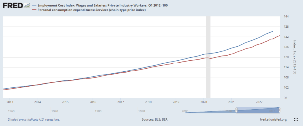
This week’s letter is about the effect of wages on inflation. In an address this week, Fed (2022) chair Jerome Powell explained the Fed’s view of the latest trends and signaled that the Fed might ease up slightly on a rate increase at its December 13-14th meeting. Friday’s jobs report had stronger than expected gains so that may temper the Fed’s willingness to ease up on the “rate brake.” In his speech, Powell cautioned that “nominal wages have been growing at a pace well above what would be consistent with 2 percent inflation over time.”
The services portion of the economy consists of mostly labor so the Fed focuses on just that sector to gauge the underlying demand for labor. In the graph below are total wages and salaries (blue line) and the services sector (red line). Both series bent upward from their pre-pandemic trends but the Fed is focused on the upward momentum of wage increases (blue line) as an underlying driver of “core” inflation.
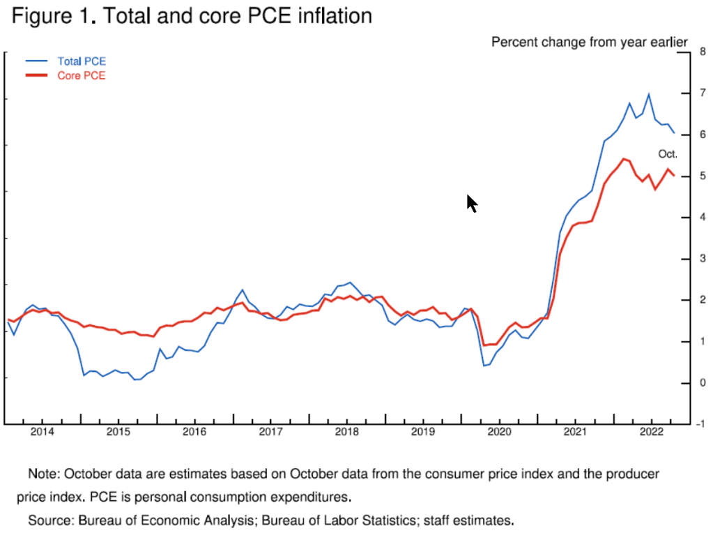
Core inflation does not include volatile food and energy prices. Those matter a great deal to consumers but the variance makes it more difficult to predict a future price path. Imagine walking a dog on a leash down a park path. The dog might dart from side to side to sample the smells along the path but the walker stays more centered on the path. An observer who could not see the path would likely watch the person rather than the dog to predict the direction they were taking. Below is a chart from Powell’s presentation.
On a long-term basis there are two trends that are likely to produce upward wage pressures. Growth in the working age population has slowed and the participation rate has declined. Since the beginning of 2021, wages have increased 11%. The labor force has increased only 3%, partly due to demographics and partly due to a participation rate that is 1% less than the pre-pandemic level. Should the trend continue, it will affect the supply of workers, causing employers to compete by paying higher wages or give up and abandon expansion plans. The first leads to persistent inflation. The second leads to a recession.
While the Fed might moderate their rate increases, history has warned not to ease up on rate increases at the first sign of slowing inflation. In the early and late 1970s, the Fed eased and inflation resumed its upward climb. It’s like relaxing the tension on a leash and the dog immediately rushes ahead. The Fed’s tools are blunt instruments, relatively easy to deploy, but lack any surgical precision. Increasing rates dampen inflation, but both have the hardest impact on low income families who will welcome the relief of lower inflation. They can expect little help from a divided Congress as it struggles to enact any fiscal policy.
I worry about the next two years. Republicans have been out of power for a century. By that I mean that voters rarely given them the full reins of power, a trifecta where the same party controls the Presidency, the Senate and the House. They held power in the 83rd Congress from 1953-1955 and again in the two years of the 115th Congress, from 2017-2019. Their longest stint was the four years 2003-2007, a time of repeated failure and scandal – the mismanagement of the Iraq war, Hurricane Katrina, the accounting and energy scandals. They are not a party that governs well because they do not respect governing, only the political power that accompanies governing. They have become a reactionary party whose strategy is a “Lost Cause” narrative familiar to the southern Democrats they absorbed into the party over the past five decades. Party leaders and conservative talk show hosts echo a constant refrain that Republicans are the last standing guardians of traditional American values. I worry because Republicans are a party who breaks things and people are more breakable in the aftermath of the pandemic.
U.S. Bureau of Labor Statistics, Employment Cost Index: Wages and Salaries: Private Industry Workers [ECIWAG], retrieved from FRED, Federal Reserve Bank of St. Louis; https://fred.stlouisfed.org/series/ECIWAG, December 2, 2022.
U.S. Bureau of Economic Analysis, Personal consumption expenditures: Services (chain-type price index) [DSERRG3M086SBEA], retrieved from FRED, Federal Reserve Bank of St. Louis; https://fred.stlouisfed.org/series/DSERRG3M086SBEA, December 2, 2022.
Hope everyone had a good Thanksgiving. This week’s letter is about a type of income that we don’t often think about, how that affects asset values and a proposal to increase homeownership. With left over buying power, people purchase assets in the hope that the buying power of the asset grows faster than inflation. There are two types of assets: those that produce future consumption flows and collectibles whose resale value increases because they are unique, desired and in limited supply. An example of the first type is a house. An example of the second type is a painting. Let’s look at the first type.
House Equals Future Shelter
A house is a present embodiment of current and future shelter. The value of that utility depends on environmental factors like schools, crime, parks, access to recreation, shopping and entertainment. These affect a home’s value and are outside a homeowner’s control. A school district’s rating in 2042 may be quite different than its current rating. Our capitalist system and U.S. tax law favors home ownership in several ways. The monthly shelter utility that a home provides is capitalized into the value of a property. Every consumption requires an income, what economists call an imputed rental income. Two thirds of homes are owned by the person living there (Schnabel, 2022) and a little more than half are mortgage free. Unlike reinvested capital gains in a mutual fund, this imputed income is not taxed to the homeowner. Let me give an example.
If the market rate for renting a similar home were $2000 a month, that is an implicit income to the homeowner. Because there is no state or federal tax on that income, the gross amount of that $2000 would be about $2400. That’s almost $30,000 a year. After monthly costs for taxes, insurance and maintenance, the annual implicit operating income of the property might be $25,000. At a cap rate of 5% (to make the math easy), the capital value of the property is $500,000. Each year, Congress requires the U.S. Treasury to estimate the various tax expenditures like these where Congress excludes certain income items from taxes. The implied income on owning a home is called “imputed rental income” and in 2021 the Treasury (2022) estimated that the income tax not collected was $131 billion. How much is that? A third of the $392 billion paid in interest on the public debt. If we did have to pay taxes on that imputed income, it would lower the value of our homes. For many decades, Congress has not dared to include that implied income.
Mutual Fund Capital Gains
Let’s return to the subject of reinvested capital gains in a taxable mutual fund held outside of an IRA or pension type account. Some of what I am about to say involves tax liability so I will state at the outset that one should consult a tax professional before making any personal buy and sell decisions. When some part of a fund’s holdings are sold, a capital gain is realized from the sale and paid to the investor who owns the mutual fund. If the investor has elected to have dividends and capital gains reinvested, the money is automatically used to repurchase more shares of the mutual fund. The balance of the account may change little but there is a taxable event that has to be included in income when the investor completes their taxes for the year. Many mutual fund holdings recognize capital gains in December.
Mutual fund companies provide the tax basis or unrealized gain/loss for each fund but often do not include that information on the statement. The unrealized gain is the price appreciation has not been taxed yet. For example, the dollar value of a fund may be $50,000 and the unrealized gain $5,000. This is more typical of a managed fund than an index fund which does not adjust its portfolio as frequently as a managed fund. If an investor were to sell the fund to raise cash, they would pay taxes on the $5,000, not the $50,000. The unrealized gain in an index fund might by 70% of the value of the fund. If the fund value is $50,000, the unrealized gain could be $35,000 and the investor would owe taxes on that amount. An investor can minimize their tax liability with a judicious choice of which fund to sell. Again, consult a tax professional for your personal situation.
Affordable Homeownership
Let’s visit an imaginary world where people do not have to pay property taxes outright. Each year they can elect to sell a portion of their property to the city or other taxing authority. Cities sometimes place tax liens on properties when a tax is not paid. This would be like a voluntary lien making the city a temporary part owner of the property until the homeowner sells it.
Imagine that a homeowner owns a home worth $400,000. For ten years, they have elected to have the city deduct an annual $2000 average property tax from the value of the home. Over the ten year period, the accrued sum is $20,000 plus an interest fee that is added to the principal sum of the tax. These voluntary tax liens would be visible to a lending institution so that the sum would lower the home’s value for a HELOC, or second mortgage. The city would report that annual amount each year as an imputed income to the homeowner and the homeowner would have to pay income taxes on it. At a 20% effective federal and state tax rate, the out-of-pocket expense would be about $480 on $2000. After the 2017 tax law TCJA, property taxes are no longer deductible so the homeowner has to earn $2400 to pay the $2000 tax outright. There is a slight change in income tax revenue to the various levels of government. When a home is sold those tax liens would be paid back to the city.
Why don’t we have such a system in place now? In the U.S. private entities own most of the capital. Some people would be uncomfortable knowing that a government authority had some legal claim to their property but they could opt out. In a pre-computer age, the accounting would have been a nightmare. Such a system is feasible today. Mutual fund companies have demonstrated that they can track the complex capital positions of their customers. Cities can do the same.
Such a system would make home ownership more affordable for a lot of people without affecting those homeowners who preferred to pay the property tax outright as we do under the current system. Investment companies would be eager to amortize those voluntary tax liens held by city governments. In the event of another financial crisis, a decline in housing prices and a rise in foreclosures, the city would be first lienholder, first in line to get paid when the property is foreclosed. Interest groups that advocate for affordable housing would be joined with investment and pension companies who wanted to underwrite the bonds for such a program.
A Capitalist System of Greater Inclusion
Some blame our capitalist system for the inequities in our society. The fault lies in us, not the capitalist system. Feudalism, mercantilism, capitalism, socialism, communism and fascism are systems of rules that embody a relationship of individuals to 1) property and the manner of production, both current and future, 2) the society, our families and communities, 3) the government that recognizes those relationships. The capitalist system is the most versatile ever invented and yes, it has been used to exclude people just as the other systems have been used to weaken some classes of people. The capitalist system can be extended to include and strengthen more of us. This homeownership policy could broaden that inclusion.
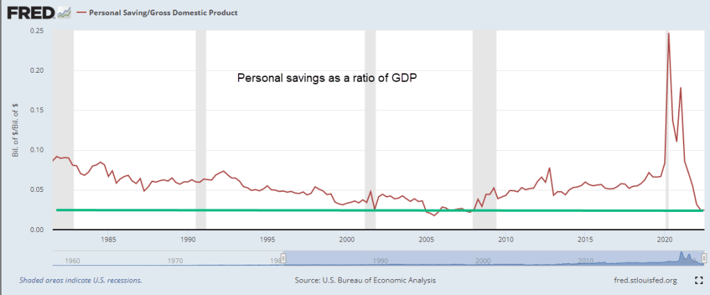
This week’s letter is about household savings and corporate profits. As a share of GDP, savings are near an all-time low while profits are at an all-time high. Elon Musk, the CEO of Tesla, appeared in court this week. No, this wasn’t about his acquisition of Twitter. It concerned a shareholder lawsuit against Tesla regarding the $50B stock option package the company awarded him in 2018. In 2019 the company’s total revenue – not profit – was less than $25B. In 2022, annual revenue was $75B. At a 15% profit margin, the company must continue growing its revenue at a blistering pace to afford Mr. Musk’s incentive pay package. Large compensation packages like this are only a few decades old. Let’s get in our time machine.
In 1994, Kurt Cobain, the 27 year old leader of the rock group Nirvana, died from an overdose of heroin. Something else was dying that year – corporations were breaking free of national boundaries and moving production to countries other than their home nation. This was the last stage in the evolution of multinational corporations, or MNCs. In earlier decades, companies had licensed or franchised their brand. Perhaps they had set up a sales office in a foreign country. Now they were becoming truly global. Fueling that expansion was an increase in equity ownership by large institutional investors. To accommodate these changes, their governance structures changed. Executives capable of leading this global growth were rewarded on a parallel with superstar sports talent. That was the conclusion of Hall and Liebman (2000, 3), two researchers at the National Bureau of Economic Research.
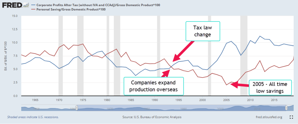
Let’s look at two series over the past sixty years – personal savings and corporate profits. If we think of a household as a small enterprise, personal savings is the residual left over from the household’s labor. Likewise, corporate profits are the residual left over from current production. In 1994, the two series diverged. Corporate profits (the blue line in the graph below) kept rising while personal savings plateaued for a decade. Each series is a percent of GDP to demonstrate the trend more easily.
Executive Compensation
In the mid-1990s, corporations began to issue a lot more stock options to their executives. Some think that a change in the tax code might have precipitated this shift in compensation. In 1994, Section 162m of the IRS code limited the corporate deductibility of executive pay to $1 million (McLoughlin & Aizen, 2018). By awarding non-qualified stock options to their executives, companies could preserve the corporate tax deduction. However, the slight tax advantage did not account for the rapid increase in options awards. Hall and Liebman found that the median executive received no stock option package in 1985. By 1994, most did. The tax change was secondary – a distraction. Institutional investors wanted more growth and more profits and companies were willing to reward executives with compensation packages similar to sports stars (Hall & Liebman, 2000, 5). Some of these superstars included Jack Welch of General Electric, Bill Gates of Microsoft, Michael Armstrong of AT&T.
Income Taxes – Less Savings
In 1993, Congress passed the Deficit Reduction Act that raised the top tax rate from 31% to almost 40%. Personal income tax receipts almost doubled from $545 billion in 1994 to almost $1 trillion in 2001. The booming stock market in the late 1990s produced big capital gains and taxes on those gains. For the first time in decades the federal government had a budget surplus. However, more taxes equals less personal savings so this contributed to the flatlining of personal savings during that period.
Household Debt Supports More Spending
During the 2000s, personal savings remained flat. On an inflation adjusted basis, they were falling. Too many people were tapping the rising equity in their home to pay expenses and economists warned that household debt to income ratios were too high. Savings as a percent of GDP fell to a post-WW2 low. As home prices faltered and job losses mounted in late 2007, people began to save more but their debt left them with little protection against the economic downturn. During 2008, personal savings began to increase for the first time in fifteen years. More savings meant less spending, furthering the economic malaise that began in late 2007.
Multi-National Corporate Profits
During those 15 years corporate profits rose steadily as companies increased their global presence. Beginning in 1994 U.S. companies began shifting production to Mexico where labor was cheaper. In 2001, China was admitted to the World Trade Organization (WTO) and production outsourcing continued to Asia. Despite the profit gains, companies kept their income taxes in check. In 2021, corporate income taxes were at about the same level as in 2004. That contributed to the rising budget deficit during the first two decades of this century.
Federal Deficit
The prolonged downturn in 2001-2003 and the financial crisis and recession of 2007-2009 put a lot of people out of work. This triggered what are called “automatic stabilizers,” unemployment insurance and social benefits like Medicaid, housing and food assistance. The federal government went into debt to pay for the Iraq War, pay benefits to people and help fill the budget gaps in state and local budgets. The tax cuts of 2003 enacted under a Republican trifecta* of government control reduced tax revenues, further increasing the deficit. During George Bush’s two terms, the debt almost doubled from $5.7 trillion to $11.1 trillion.
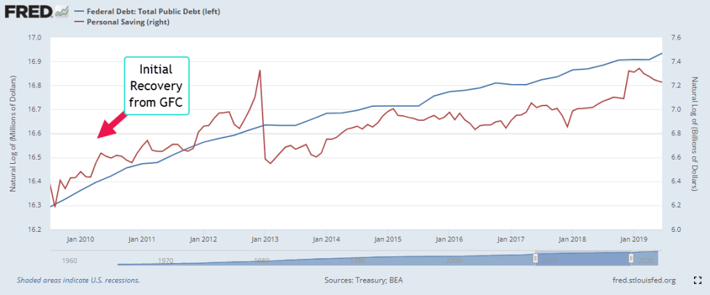
In coping with the recovery from the financial crisis, the government added another $8.7 trillion to the debt. That negative saving by the government helped add to the personal savings of households but too much was spent on just getting by. Following the Great Financial Crisis (GFC), the trend of the government’s rising debt (blue line below) matched the trend in personal savings (red). Sluggish growth and lower tax revenues caused the two to diverge. While the debt grew, personal savings lagged.
Before and During the Pandemic
Following the 2017 tax cuts enacted under another Republican trifecta, personal saving rose, then spiked when the economy shut down during the pandemic and the federal government sent stimulus checks under the 2020 Cares Act. In the chart below, notice the spike in debt and savings. By the last quarter of 2020, personal savings had risen by $600 billion from their pre-pandemic level of $1.8 trillion. In late December, President Trump signed the $900 billion Consolidated Appropriations Act (Alpert, 2022) but that stimulus did not show up in personal savings until the first quarter of 2021. In March 2021 President Biden signed the $1.7 trillion American Rescue Plan. Personal savings rose $1.6 trillion in that first quarter, the result of both programs.
After the Pandemic
Some economists have said that the American Rescue Plan was too much. In hindsight, it may have been but we don’t make decisions in hindsight. As more schools and businesses opened up, households spent far more than any extra stimulus. They spent $1.2 trillion of savings they had accumulated before the pandemic and savings are now at the same level as the last quarter of 2008 when the financial crisis struck. Thirteen years of cautious savings behavior has vanished in a few years. On an inflation-adjusted basis, personal savings is at a crisis, almost as low as it was in 2005. In the chart below is personal savings as a ratio of GDP.
The Future
In the past year savings (red line) and corporate profits (blue line) have resumed the divergence that began almost three decades ago. Profits were 12% of GDP in the 2nd quarter of 2022. Savings is near that all time low of 2005. Rising profits benefit those of us who own stocks in our mutual funds and retirement plans. However, the divergence between the profit share and the savings share is a sign that the gap between the haves and the have-nots will grow larger.
Hall, B. J., & Liebman, J. B. (2000, January). The Taxation of Executive Compensation – NBER. National Bureau of Economic Research. Retrieved November 19, 2022, from https://www.nber.org/system/files/chapters/c10845/c10845.pdf. Interested readers can see Moylan (2008) below for a short primer on the recording of options in the national accounts. Until 2005, these options were recorded as compensation for tax purposes but not recorded on financial statements so they did not initially affect stated company profits.
October’s CPI report released this week indicated an annual inflation of 7.7%, down from the previous month. Investors took that as a sign that the economy is responding to higher interest rates. In the hope that the Fed can ease up on future rate increases, the market jumped 5.5% on Thursday. Last week I wrote about the change in the inflation rate. This week I’ll look at periods when the inflation rate of several key items abruptly reverses.
Food and energy purchases are fairly resistant to price changes. Economists at the Bureau of Labor Statistics (BLS) construct a separate “core” CPI index that includes only those spending categories that do respond to changing prices. It is odd that a core price index should exclude two categories, food and energy, that are core items of household budgets.
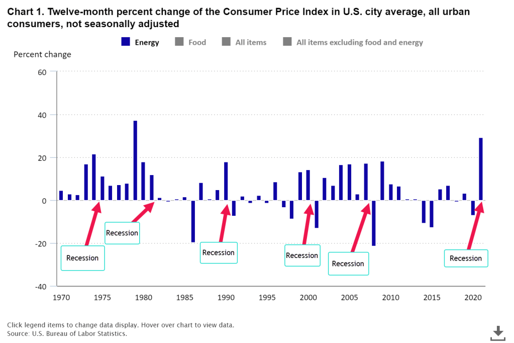
Ed Bennion and other researchers (2022) at the BLS just published an analysis of inflationary trends over several decades. Below is a chart of the annual change in energy prices. Except for the 1973-74 oil shock, a large change in energy prices led to a recession which caused a big negative change in energy prices.
We spend less of our income on food than we did decades ago so higher food prices have a more gradual effect, squeezing budgets tight. Lower income families really feel the bite because they spend a higher proportion of their income on food. In the graph below a series of high food price inflation often precedes a recession. Unlike energy prices, there is rarely a fall in food prices. Following the 2008 financial crisis, food prices fell ½% in 2009. It is an indication of the economic shock of that time.
Let me put up a chart of the headline CPI (blue line) that includes food and energy and the core inflation index (red line) which does not. Just once in 75 years, during the high inflation of the 1970s, the two indexes closely matched each other. Following the 1982-83 recession, the core CPI has outrun the headline CPI.
A big component of both measures of inflation is housing. The Federal Reserve (2022) publishes a series of home listing prices calculated per square foot using Realtor.com data. You can click on the name of a city and see its graph of square foot prices for the past year. You can select several cities, then click the “Add to Graph” button below the page title and FRED will load the graph for you. Here’s a comparison of Denver and Portland. They have similar costs.
The pandemic touched off a sharp rise in house prices in both cities. Denver residents have attributed the big change to an influx of people from other areas. However, Census Bureau data shows that the Denver metro area lost a few thousand people from July 2020 to July 2021 (Denver Gazette, 2022). In the decade after the financial crisis, there simply wasn’t enough housing built for the adults that were already here.
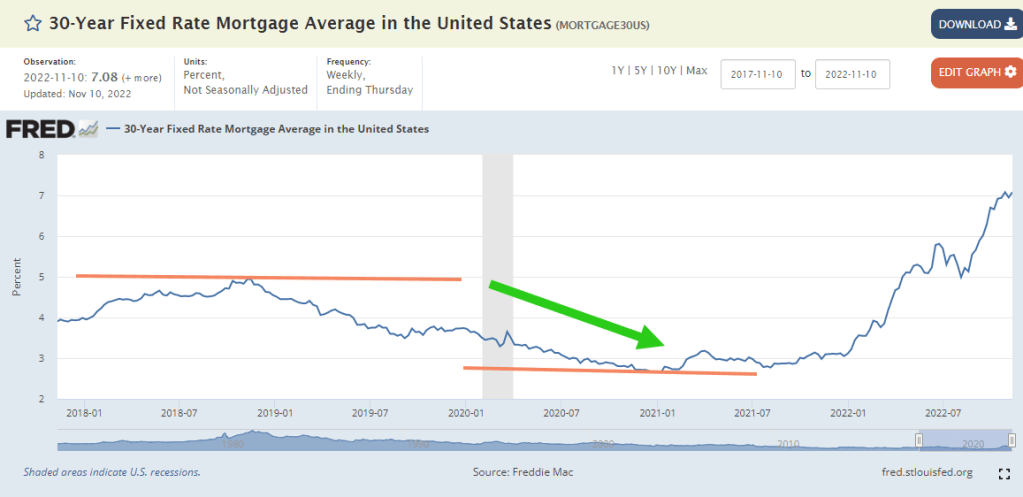
The surge in home buying has not been in population but in demographics. As people approach the age of 30, they become more interested in and capable of buying a home. The pandemic helped boost home buying because interest rates plunged from 5% in 2018 to 2.6% in 2021.
Record low interest rates enabled Millennials in their 20s and 30s to buy a lot more home with their mortgage payment. That leverage caused housing prices to rise. A 30-year mortgage of $320K has a monthly mortgage payment of $1349 at 3%. At 5%, it is $1718 and at 7% it rises to $2129. Ouch!
Rising rental costs and home prices drive lower income families to less expensive areas in a metro area or entirely out of an area. Declining public school enrollment has forced two Denver area counties to announce the closing of 26 schools and transfer them to other schools (Seaman, 2022). As the number of students decreases, the schools infrastructure costs do not change, increasing the per student costs. Buses have to be maintained, drivers paid, schools staffed with guards, cafeteria staff, janitors and administrative personnel. Once schools are shuttered, the building may be sold and converted to other uses, either residential or commercial. The public schooling system is like a large ship that takes some time to change course.
During our lifetimes we experience many changes. They can happen quickly or emerge over time. The effects may be short lived or last decades. Families are still living with the consequences of the financial crisis fourteen years ago. Carelessly planned urban development isolates the residents of a community. The social and economic effects can last several generations. As we grow older, we learn to appreciate William Faulkner’s line, “The past is never dead. It’s not even past.”
Many people compare today’s inflation with that of the 1970s. A better comparison might be with a much earlier period. This week’s letter will be about the change in the inflation rate. Inflation is like the speed on a speedometer. If I accelerated from 50 to 60 MPH over a certain time period, perhaps 10 seconds, the change in the speed is 10 MPH. The time period I’m looking at is one year. If inflation rose from 1% to 5% in a year’s time then the change is 4%.
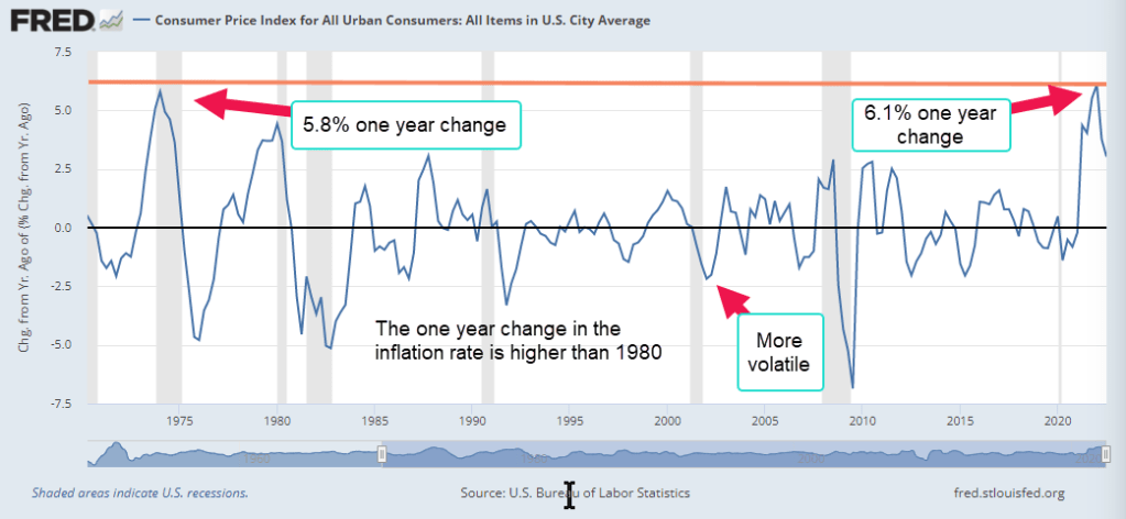
I’ll start with the current year. The one year change peaked at 6.1% in the first quarter of 2022. As the Fed raised rates, that change moderated. It’s like accelerating to 60 MPH and realizing that the speed is over the speed limit and reducing speed by easing up on the gas pedal or braking.
Most of the time the inflation rate changes by less than 2% up or down. During and after recessions it can become more volatile. In 1980, inflation soared above 14% and the one year change peaked at 5.8%, slightly less than our recent experience.
There has only been one time in the past 70 years when the inflation rate rose faster than today. That was in 1951, shortly after the Korean War began. For the first six months of 1950, prices sank – deflation – then war was declared in June 1950 and the U.S. again ramped up defense production. The one year change in inflation peaked above 10% as Federal defense spending shot up 45%.
If you would like to explore this period in more detail Tim McMahon (2014) presents 1950s inflation data in an easy to read format. A hundred years ago, a period of persistent deflation – not inflation – followed the last pandemic. See Tim’s second link below. The Federal Reserve was still fairly new and the U.S. and European nations had adopted a gold standard that would eventually lead to the Great Depression. That’s another story. Today the world’s commerce is interlocked and pandemic shutdowns continue to deliver a series of supply shocks. Getting policy right is more difficult when circumstances are this unusual.
Volatile Inventories
Inflation rises when there are inadequate resources to meet demand. In 2021, real private gross domestic investment rebounded quickly, rising almost 32% on an annualized basis in the 4th quarter. One component, inventories, was responsible for much of that surge. Even under normal conditions, this series is a volatile component of GDP (BEA, 2019) and the BEA publishes a figure called Final Sales of Domestic Product which excludes the change in inventories. Real final sales is approximately close to inflation-adjusted GDP.
During the pandemic manufacturing and retail goods sat in container ships off the port of Los Angeles and other ports. While the goods were in transit, they were not added to inventories. In the 2nd quarter of 2021, businesses began to open again but the ports were slow to unravel their logjams. Empty truck containers sat in parking lots and on neighborhood streets near the L.A. port while ships waited in line out on the water.
Sales surged as economy reopened
In the 2nd quarter of 2021, real final sales increased 2%, finally reaching pre-pandemic levels. In the first half of the year, real food and service sales shot up 10%. Normally that increase would occur over three years. However, within months that initial surge subsided. Over the next two quarters, real final sales barely increased. Real food sales declined slightly. This confirmed a temporary response to a post-pandemic recovery. With so many items out of stock, customers were willing to pay higher prices to get products. Some businesses had orders shipped from Asia by air. In the 4th quarter 2021, the floodgates opened and real private inventories rose by a record $197 billion.
Profits Surge
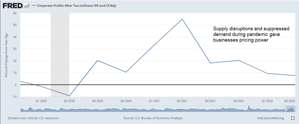
Real retail and food services sales fell slightly. In the last six months of 2021 inflation topped 5% but people were not buying and selling more stuff. Where were the price pressures? During the inflationary second half of the 1970s, profits increased a whopping 12% per year in those five years. In 2021, corporate profits rocketed up. Supply disruptions and repressed demand during the pandemic gave businesses pricing power. In 2021, corporate profits increased 18%. If demand was relatively flat, that pricing power had to fade but profit growth was still strong in the first quarter. Like the 1970s, rising corporate profits and pricing power were major contributors to inflation. This week the House Committee on Oversight and Reform (2022) came to a similar conclusion. What is the source of that pricing power?
War in Ukraine
In February 2022, Russia attacked Ukraine, sending energy prices higher. XLE, a broad energy ETF, gained 35% by early March. Two months later, the BEA reported another record rise in real private inventories of $214 billion. However, real final sales fell 2.5%. Some economists pointed to low unemployment and rising wages but ECI wages of private workers were on the same trend as before the pandemic when inflation was low. Most of the rise in the inflation rate was in housing, food and energy prices. The pandemic and low interest rates had contributed to the rise in housing costs. The war in Ukraine was responsible for volatile energy prices. There was no increase in real food sales but food prices were rising. Four large meat producers had profit growth of 134%, the committee reported.
The Puzzle
Historians still argue about the causes of World War I a century ago. Economists still cannot agree on the inflation mechanism of the 1970s. Contributing causes were rising corporate profits, shifting demographics in the work force, oil supply shocks, a shift in the international monetary regime and an evolving trans-global economy in the post war era. Economists do agree that it was a gestalt of market, fiscal and monetary forces, complicated by geopolitical and policy shocks that shaped expectations of future inflation. When people expect further price increases, they buy more now, aggravating inflationary pressures. Those expectations helped entrench inflation in the economy of the 1970s. Paul Volcker, chairman of the Fed in the late 1970s and early 1980s, raised interest rates so high that it wrung inflation out of the economy but at great economic cost to many families. The high interest rates caused two recessions, one of them the worst since the Great Depression.
The Korean War
In answer to the surge of inflation in 1951, the Fed raised rates slightly but rates stayed below 2%. The government did the heavy lifting. In September 1951, President Truman started a regime of wage and price controls administered by the Economic Stabilization Agency (ESA) and Wage Stabilization Board (WSB). There were loud protests against the controls and President Eisenhower ended them after he took office in 1953. Several months later the Korean War ended. In 1971, President Nixon instituted wage and price controls and demonstrated the failure of controls. Monetary policy is the weapon of choice to combat inflation but rising rates disproportionately affect the most vulnerable workers.
Conclusion
Infrequent events are an intersection of many factors that make each one unique. As economists pull apart the tangle of causal narratives, they develop new theories or modify existing ones. Economists usually cling to a favorite – either supply or demand. I’m watching profit growth. If Republicans take the House and possibly the Senate in the coming election, they will try to further enhance corporate profits at the expense of social programs like Medicare and Social Security. Republicans continue to sell a “trickle down” narrative but decades of evidence shows that the trickle is but a few drops. What goes to the top stays at the top.
This week’s letter is a detour into political branding and public opinion. In interviews with voters, I often hear “I am a [‘Democrat’ or ‘Republican’ or ‘Independent’ here].” It is not unusual to hear the same association with a religion as in “I am a Lutheran” or “I am a Catholic.” These identifications begin when we are young, extending the reach of our sense of self outside the family (Miller & Shanks, 1996, 120). These party affiliations are not mental straitjackets by any means. As we come of age, we form a unique set of values and group identifications and may adopt a party affiliation different from our parents. This can make for some uncomfortable conversation at the Thanksgiving dinner table.
We may self-identify with a party because we are not like those people in that other party. Political and cultural scientists have a term for this process of stereotyping people – othering. We might identify as an Independent voter because we are not a crowd follower like those Democrats and Republicans. We are discerning voters who study the issues and candidates before we vote. That is also a form of othering.
Magleby et al. (2011, 247) found that many self-identified Independents are leaners, leaning toward one party or the other, and are more engaged in political issues. In Presidential elections from 1952 to 2008, Republican leaning Independents voted almost 78% of the time, about the same as Weakly Partisan Republicans. Democrat leaning Independents showed the same behavior. Truly Independent voters who are not leaners have less interest in politics and voted only 63% of the time. In recent years, that percentage has dropped to 53%.
Our party system treats people as though they were computer switches – on or off, left or right. Many of us have graduated value systems that cannot be simplified like a logic gate on a circuit board. Citizen initiated ballot measures reveal that complexity. Many states have citizen initiatives, allowing interest groups to put legislative proposals on the ballot after collecting a number of verified signatures. A voter might be for a proposal to provide free lunches for all students but does not like the way the program is funded and votes NO. The ballots contain only the two choices – YES or NO. Consider a ballot that allowed a voter to represent their actual opinion. A neutral position would be 0. A voter could vote for the proposal on a scale from 1 to 5, or against the proposal on a scale of -1 to -5. We have the technology. Why don’t we have the ballots?
Despite evidence to the contrary, some Republicans voice distrust with voting machines and want to return to the days when paper ballots were counted by hand. They ignore the extensive testing procedures that their own Republican state legislatures conduct (NCSL, 2021). Republican voters who say they doubt the integrity of the vote are, in effect, doubting the honesty of their own party’s legislators whom Republican voters elected. The story is so illogical that Democrats have been unable to tell a narrative that would replace the Republican fairy tale. That is the genius of the Republican political narrative.
In Colorado, a Republican candidate for governor is one of more than a dozen Republican candidates around the country who have been telling outlandish stories that the schools are teaching children to identify as cats and use litter boxes (Klamann, 2022). If the illogical story with the voting machines caught fire with some voters, particularly Q-Anon believers, why not adopt the same strategy and try other bizarre stories? The stories are political hornets, designed to keep Democrats occupied by reminding people of actual facts. In the early 1950s, Republican Senator Joe McCarthy kept Democrats preoccupied with tall tales of Communists lurking behind every bush in Washington and Hollywood. Alex Jones emulates that McCarthyite cruelty and craziness.
Some Republican candidates celebrate othering and continue to build the Republican party on bias and exclusiveness. Southern Democrats successfully employed that strategy for 100 years after the Civil War. Former First Lady Michele Obama encouraged people to take the “high road” and not give into hate rhetoric. Lies, wild accusations of socialism and staged Tea Party rallies contributed to a historic loss of Democratic House seats in the 2010 midterms. In our winner-take-all electoral system, there is only one road to victory and political power. It is neither high nor low.
Democracy thrives on open distrust, on bold lies and the histrionics of political candidates and their supporters. Few Chinese dare to voice distrust with their leader, Xi Jinping. At the gathering of the CCP Congress this month, there was no wild gesticulating or shouting like there is at American political conventions and sometimes at State of the Union addresses. Americans treat politics like a rodeo, swooping and hollering. Chinese leaders look profoundly serious. In both countries, people are getting hurt, jailed and isolated but the American system is entertaining.
Magleby, David B, Candice J. Nelson, and Mark C. Westlye. 2011. “The Myth of the Independent Voter Revisited.” In Facing the Challenge of Democracy: Explorations in the Analysis of Public Opinion and Political Participation, eds. Benjamin Highton and Paul M. Sniderman. Princeton, NJ: Princeton University Press. essay, 238–64.
Miller, Warren Edward, and J. Merrill Shanks. 1996. The New American Voter. Cambridge (Mass.): Harvard University Press.
This week’s letter is about taxes and income. Each month, the Federal Reserve (2022) releases an estimate detailing how people spend their money and the sources of their income. I was surprised that 17% of personal income is from government transfers like Social Security and other programs. This is 2% more than the income people receive on their assets. A bit of history for context.
In the 1960s, 2/3 of income was from wages and salaries. Each decade, the wages and salaries component declined 5% until this past decade when wages and salaries were just 50 cents out of every dollar of income.
A greater portion of employee compensation shifted from discretionary income to dedicated non-taxable benefits like health care insurance and pensions. In the early 1960s employer benefits were 10% of wages and salaries. Now they are 21%. Despite the rise in the non-taxable share of compensation, workers give up more out of their paychecks to taxes.
A growing share of income goes to FICA taxes
In 1960, workers paid 6% of their paychecks to FICA taxes. The Medicare program, about 20% of our FICA taxes today, would not be enacted until 1965 when President Johnson ushered in his Great Society programs. Within five years analysts realized that lawmakers had wildly underestimated the costs of the program. By 1980, increases in Social Security and Medicare taxes increased the FICA portion to 12% of paychecks. Today, workers pay 15% of their paychecks in FICA taxes (see note).
In 1960, all other taxes were 11% of total income in 1960, had climbed to almost 13% in 1980 then to over 14% by the year 2000 and are now 15% of total income. In the past twenty years, the rich have paid a growing share of income taxes but their effective tax rate has changed little. Why? When lawmakers put a heavier burden on rich people, they lobby for legal income exclusions and Congress obliges.
Top 10% pay a growing share of income tax
In 2001, the top 1% paid 33% of income taxes. In 2019, they paid 39% (IRS, 2022). In 2001, the top 10% (the Tennies, I’ll call them) paid 64% of personal income taxes. In 2019, they paid 71%. Whether it is the super-rich or the rich, their share of income tax has grown by 6 -7%. That’s not the end of the story.
Growth in incomes of the top 10% is far higher
The Tennies have seen their share of gross income increase from 42.5% in 2001 to 47.3% in 2019, a gain of almost 5 percentage points. They have paid a rising share of the nation’s income taxes but the rise in taxes is less than the rise in personal income (BEA, 2022). In the 2001-2003 period the income tax paid by the Tennies averaged 5.6% of national personal income. In the 2017-2019 period, that tax share was 6.3%, a difference of just .7%. It is a cheap price to pay for a 5% gain in the nation’s total income.
Effective Tax Rate of the top 10% is steady despite rise in Income
In the 2001-3 period the Tennies averaged an effective tax rate of 13.5%. In the 2017-19 period, that effective rate had declined to 13.2% despite a 2% rise in the top marginal tax rate from 35% in 2001 to 37% in 2019. Raising the marginal tax rate on the highest income brackets has little net effect yet it was a campaign issue for Mr. Biden and many Democrats. Political scientists call it position-taking.
The party of no taxes produces higher deficits
Despite their rhetoric about reducing the deficit, Republicans have adopted a no new taxes on anyone pledge that ensures the deficit will get worse. True to form, the budget deficit has grown more under Republican administrations over the past four decades. The party also has a record of slower economic growth but that is mostly due to the two terms of the George Bush administration. Mr. Bush’s failures caused many Republicans to abandon more mainstream Republican values and adopt a mean spirited attitude of radical defiance exemplified by the Tea Party and the Republican Study Committee.
Action requires Compromise
The “Just Say No” Republican factions permit little compromise so the party cannot get significant legislation passed. In the first year of Mr. Trump’s Presidency, Republicans held all three legislative bodies but were stymied by their internal squabbles. In November of 2017, they hastily assembled the corporate tax reform package, TCJA, to show their constituents that they were capable of legislating and to give Mr. Trump some accomplishment that he could tweet about.
A look ahead
If Republicans take control of the House after the upcoming elections, we can expect more of the same dysfunction under Speaker Kevin McCarthy. Libertarians in the Republican Party want a limited role for the federal government as specified in Article 1, Section 8 of the Constitution. They have little tolerance for national abortion laws and other bullying social legislation that Republicans have promised. The uncompromising factions within the Republican Party ensure that the party cannot govern. They are like drivers in a car with a manual transmission who don’t know how to clutch and shift. Democratic lawmakers, on the other hand, drive down the road, focused on staying perfectly centered between the white lane markers of equality and equity. The rich benefit when party leaders cannot assemble a cohesive coalition of interest groups and voters. The economic interests of the top 10% are protected when voters remain fragmented. Party elites and partisan interest groups speak in languages that are understandable only to a narrow constituency. By promoting dissension, social media has helped create a Tower of Babel.
BEA: U.S. Bureau of Economic Analysis, Personal Income [PI], retrieved from FRED, Federal Reserve Bank of St. Louis; https://fred.stlouisfed.org/series/PI, October 19, 2022.
Federal Reserve. (2022). Personal income and its disposition. FRED. Retrieved October 19, 2022, from https://fred.stlouisfed.org/release/tables?rid=54&eid=155443&od=#. The FICA tax percentage includes the employer and employee portion of the tax. The employee effectively bears the burden of the entire tax.