Easter Egg

April 5, 2015

On this Easter Sunday, Christians celebrate the Resurrection of Jesus, Jews observe Passover, basketball fans await the final contest of the Final Four and baseball fans look forward to the start of the new season.  After Friday’s disappointing report of job gains in March, investors might be wondering what will happen Monday when markets in the U.S. reopen following Good Friday.  In overseas markets, yields on the 10 year Treasury bond fell on the employment news.  Job gains that were about half of expectations helped allay fears of a June rate increase.  We may see a positive response from both the bond and equity markets on Monday as the time table for rate increases might start in September.  On the other hand, the weekend might allow more rational judgment to prevail. One month’s disappointment does not a trend make.  Year over year gains in employment are especially strong.

April is usually a good month in the stock   market.  Since breaking the 2000 mark in August, the index has neither gained or lost much ground.  Gains in the technology companies that are included in the SP500 (Apple, for example) have been offset by losses in the oil sector of the SP500 (Exxon, Chevron, for example).  Long term Treasuries (TLT) have risen 10% in the past six months, despite the prospect of rising interest rates in 2015.

ICI reports that domestic long term equity mutual funds had an outflow of about $8 billion in March. Investors have not abandoned equity funds by any means but have changed focus. During this past month, $14 billion flowed into world equity funds.   Bond funds continue to post strong inflows – $10 billion in March.

The boomer generation amassed a lot of pension promises through their working years.  Pension funds must balance both equity and bond risk in their investment portfolios  and yet try to meet their assumed growth rates of 7% – 8%.  Caught on the horns of this dilemma, pension funds straddle both the equity and bond markets.  During the past ten years, many have become underfunded because they have not been able to match their projected growth rates.   This delicate balance of risk and reward sets the stage for a catastrophic decline in response to even a relatively small monetary shock because pension funds can not afford to wait out another three or four year decline.  Too many boomers will start cashing in those promises accumulated during the past decades.

The relatively low number of new jobs created in March was probably due to the severe winter in the eastern part of the country.  The BLS revised downward their previous estimates of employment gains in January and February.  Even with the downward revisions and this past month’s relatively anemic 126,000 gains, the average for the quarter is still about 200,000 per month, a particularly strong figure when one considers the impact that plummeting oil prices have had. In the first 3 months of this year, companies in oil and gas exploration have shed 3/4 of the jobs added during all of last year.  The strong dollar makes U.S. exports more expensive and hurts manufacturing.  The employment diffusion index in manufacturing industries dropped below 50, a sign that there is some contraction in the 83 industries included in this index.  However, March’s Manufacturing Purchasing Managers Index showed some slight expansion still and employment in manufacturing is still strong.  Across all private industries, the diffusion index remains strong at 61.4.

Fed chair Janet Yellen has repeatedly said that interest rate decisions will be based on data.  If the data of subsequent months show a resumption of strong growth, an interest rate increase at the FOMC meeting in late July could still be in the cards.  The CWPI composite built on the PMI anticipated a declining trend in growth this winter and spring before resuming an upward climb.  When the non-manufacturing  PMI is released this coming Monday, I’ll update that and show the results in next week’s blog.  Based on the numbers already released, I do anticipate a further decline in March then an evening out in April.  The particularly strong dollar  has cast some doubt on growth predictions, particularly in manufacturing. Both oil and the dollar have made sharp moves in the previous months and it is the rate of change which can be disruptive in an economy.

**********************

Unemployment

New claims for unemployment were the lowest since the spring of 2000, just as the bubble of the dot-com boom began to deflate.  As a percent of those working, this is the third time since WW2 that new claims have reached these very low levels.  The last two times did not turn out well for the economy or the stock market.

**********************

Oil

Going back through some old notes.  Here’s an October 2009 article where Deutsche Bank estimates the price of oil at $175 in 2016.  2009 was just about the time that newer techniques in horizontal drilling were being developed.  The fracking boom was just about to get underway.  Whether you are an investor or a second baseman, the future is tough to figure out so stay balanced, stay prepared and keep your knees bent.

New Year, No Fear

January 4th, 2015

As the calendar flips from December to January, some favorite activities are predictions for the coming year and reviews of the past year.  Here are a few predictions I’ve heard in the past few weeks:

“We think oil will continue to drift downwards as global demand slackens.”

“We think long term Treasuries will continue to show strong gains in the coming year.”

“Output remains strong, and the labor market continues to strengthen.  We expect further gains in the stock market this year.”

“We expect gold to find a bottom in the $900 to $1000 range and we will be initiating a long position at that time.”

Predictions are foolish, of course.  They are too certain.  An expectation is a bit more sober, a pronouncement of a probability.  Did anyone hear these expectations at the beginning of 2014?

“Oil prices will decline by 40% this year.”

“We expect long term Treasuries to gain 25% in 2014.”

“We expect the euro to fall to a 4-1/2 year low against the dollar.”

I don’t remember any of those predictions at the beginning of 2014.  So here’s my expectation – er, prediction: in 2015, I will be surprised by some of the events that will unfold.

If that doesn’t satisfy your prediction craving, here are several – let’s call them guesstimates – of SP500 earnings and price predictions in 2015.

*********************

Blue Light Specials

As I mentioned a few weeks ago, there are a few stock sectors that are “on sale,” selling below their 200 week, or 4 year average.  Falling gas prices in the last half of 2014 have had a negative impact on energy stocks (XLE, VDE).  Selling below their 200 week averages in December, both ETFs are hovering at their 200 week average.  The 50 week average is above the 200 week average, indicating that this is, so far, a relatively short term trend.

Emerging markets have been in the doldrums for a year and a half.  The 50 week average is just about to cross above the 200 week, signalling that the downturn may have exhausted itself.

The mining sector (XME) is down – way down.  The 50 week average is below the 200 week average and current prices of this ETF are below the 50 week average.  The mining sector can be quite cyclical but could be quite profitable in the next six months.

In the summer of 2011, the oil commodity ETF USO lost a third of its value.  In the melt down of 2008, it lost 75% of its value, falling from $115 down to near $30.  This week USO broke below $20, losing half of its value since July.  Since September 2009, shortly after the official end of the recession, the 50 week average has been trading in a range of $34 to $38, and is currently at the low point of that five year range.  While this may not be appropriate for a casual investor, it might be worth a look for those with some play money.

Other sectors – industrials, materials, finance, health, technology, consumer staples, consumer discretionary, retail and utilities – are above both their 50 and 200 week averages.

*********************

Happiness Is An Open Wallet

The Conference Board’s Consumer Confidence gauge rose still further above 90 in December.  At some time in the distant past, in a year called 1985, all the people were happier than they are today.  That long ago time became the benchmark 100 for this index.  The index number is less important than the trend of confidence – whether it is rising, falling or staying the same.

The Case Shiller 20 City Home Price Index for October showed a 4.5% yearly gain.  The double digit gains of last year and the first six months of 2014 were unsustainable.  However, I would be concerned if this continues to fall toward zero, indicating a serious softening of demand, or a lack of affordability or both.

***************************

The non-SP500 World

The SP500 index, composed of the 500 largest companies in the U.S., was up 11.4% for 2014. An index of mid, small and micro-cap companies was up a more modest 7.1% (Standard Poors) for the year.  An index of REITs was up 25.6% in 2014 after stalling during much of 2011, 2012 and 2013. I was surprised to learn that during the past twenty years, REITs outperformed the SP500.

Conventional wisdom holds that rising interest rates are bad for REIT stocks.  A study of REIT performance shows that the impact is less than most investors think. In addition, the income growth generated by REITs has outpaced inflation in all but one out the past 15 years. VNQ and RWR are two ETFs in this market space.  VNQ has a 10 year return of about 9%, RWR a bit less.

***************************

Social Security

The Social Security program depends on current taxes to pay current beneficiaries.  In per person inflation adjusted dollars, the federal government collects twice the amount of money it did forty years ago.  Per person revenues have almost caught up to the levels of 2006.

The problem is that there are a lot of people starting to retire.  Politicians of both parties have spent the excess social security taxes collected in the past decades.  Last week I asked what you would do if the stock market lost 30% of its value.

This week’s sobering question for those in or near retirement:  what would you do if social security payments were reduced, or means tested?  With the stroke of a pen, Congress could reduce the maximum monthly benefit from $2533 to say $2100.  This would affect a relatively small percentage of voters, those with higher incomes, a favorite target for benefit cuts.  Perhaps you are taking care of an ailing child or parent and need the income.  You might submit a 4 page form listing your pensions, IRAs, the assessed value of your home and any mortgage you had against the house, your mutual funds, stocks and bonds.  Using a complex formula to factor in your age, special circumstances, the cost of living index in your area and the total of your assets, the Social Security Administration would calculate your monthly benefit.  Can’t happen here in the land of the free, home of the brave?

New Directions

December 28th, 2014

Emergency Plan

Let’s say you have $60 invested in the stock market.  You have $30 invested in bonds and $10 sitting in your savings account, for a total of $100.  This is essentially a 60/40 stock/bond mix. You do not rely on your investments for current income.

Some crisis unfolds, sending shock waves through global markets.  Within a month, the stock market loses 30%.  Bonds have gone up 10% as investors flee to safety.  Financial soothsayers are predicting further stock losses, perhaps as much as 50%.  Others are saying that the market has bottomed.

Your stock portfolio has lost $18 (30% of the $60).  Your bond portfolio has gained 10% or $3.  Your portfolio is now valued at $42 stocks, $33 bonds, $10 savings, a 50/50 mix of stocks/bonds.

Now, let’s add some historical context. From 1968 to 1982, a period of fourteen years, there was no change in the SP500.  From 1982 to 2000, the SP500 rose 1400%.  Then from 2000 to early 2013, almost thirteen years, there was no change in the SP500.  Yes, it’s only been a year and a half since the market regained those levels of 2000.

So, what would you do?  Do you:

A)  Invest the $10 in savings to bring you back closer to your original allocation mix of 60/40 stocks/bonds.

B) Stick to allocation goals.  Keep the $10 tucked away in savings for emergencies, sell some bonds and buy stocks to get closer to your allocation goals.

C) Change your allocation mix.  Cut your losses by selling the stocks you own and buying the better performing bonds.

D) Shrug and make no changes.  Turn on the game and order a pizza. The stock market will rebound in due time and automatically rebalance your portfolio on its own.

E)  Freeze, not knowing what to do.  Yes, not knowing what you would do is a game plan, a choice.  Perhaps its not the best plan but it is often one chosen as the default.

Now, run that same scenario, changing only one thing. You rely on your investments and savings for half of your current income.  Now what do you do?

Was the past year and a half the beginning of an eighteen year run up in prices similar to the 1982 – 2000 period?  Could the SP500 index, currently trading near 2100, be valued at 21000 (1500 * 1400%) in 2032?  Maybe.  Could 2014 be the last year in the previous flat cycle so that the market drops 25% to the 1500 level of 2000 and 2007?  Maybe.

*******************************
GDP
The third estimate of 3rd quarter GDP growth was a strong 5% on an annualized basis, more than offsetting the weak 1st quarter of this year. On a more sobering note, it is only in the past six months that per person GDP has firmly surpassed 2007 levels.
GDP is a measure of tradeable goods and services in an economy.  There is much important human activity that is not measured in GDP so it is far from perfect.  If you want perfect, go to the universe next door. Per person GDP growth below 1% causes concern among traders, money managers, economists and policy makers.  This year per capita growth is a healthy 2% – not robust but respectable.  
Contributing to GDP growth in the third quarter was a 4% yearly increase in federal government spending, more than double the rate of inflation.
*******************************
Oil 
Monday’s meeting of the OPEC members left little doubt that Saudi Arabia is content to let the price of oil fall as low as natural supply and demand might take it.  They said they would not consider production cuts until oil went as low as $20 a barrel, about a third of what oil is currently trading at, and a fifth of its price in 2013.  This rhetoric was aimed directly at two non-OPEC members, the U.S. and Russia, warning both countries that the Saudis intend to keep their leadership position in the international oil market.
Missouri was the first state to report an average price per gallon of gas that was lower than $3.  Others are sure to follow.  A few weeks ago an EIA administrator testified before Congress, revealing a number of dramatic shifts in U.S. oil production, consumption and import.  Once the largest importer of petroleum products, the U.S. is now the world’s largest exporter.  Despite falling oil prices, the EIA expects production to increase 10% in 2015.  

Year In Review

January 5, 2013  2014

The start of any year presents an opportunity for reflection on the past year as well as the upcoming one.  At the start of the year, few, if any, analysts called for such a strong market in 2013.  The S&P500 closed the year at 1850, a 30% gain. After a correction in May – June of this year, the index rose steadily in response to better employment data, industrial production, GDP increases, and the willingness of the Federal Reserve to continue  buying bonds and keep interest rates low.

I was one of many who were mildly bullish at the beginning of the year but got increasingly cautious as the index pushed past 1600.  Yet, month after month came not only positive or mildly positive reports but a notable lack of really negative reports.  Leading economies in the Euozone, teetering on recession, did not slip into recession.  Fraying monetary tensions in the Eurozone did not explode into a debt crisis.  China’s growth slowed then appeared to stabilize.  Although the attention has been on the Eurozone the past few years, the sleeping dragon is the Chinese economy, its overbuilt infrastructure, the high vacancy rate in commercial buildings in some areas of the country and the high housing valuations relative to the incomes of Chinese workers.

A year end review is an exercise in humility for most investors.  Some fears were unfounded or events unformed which confirmed those fears.  People are story tellers – stories of the past, imaginings of the future.  An investor who keeps all their money in CDs or savings accounts is predicting an unsafe investing environment for their savings.

Perhaps the best strategy is the one that John Bogle, the founder of Vanguard, advocates.  He doesn’t try to predict the future or be the best investor.  He aims for that allocation of stocks, bonds and other investments that, on average, forms a suitable mix of risk and reward for his goals, his age and the financial situation of his family.  He looks at his portfolio once a year.  I do think that a good number of individual investors had adopted the same outlook as Mr. Bogle advocates – until the 2008 financial crisis.

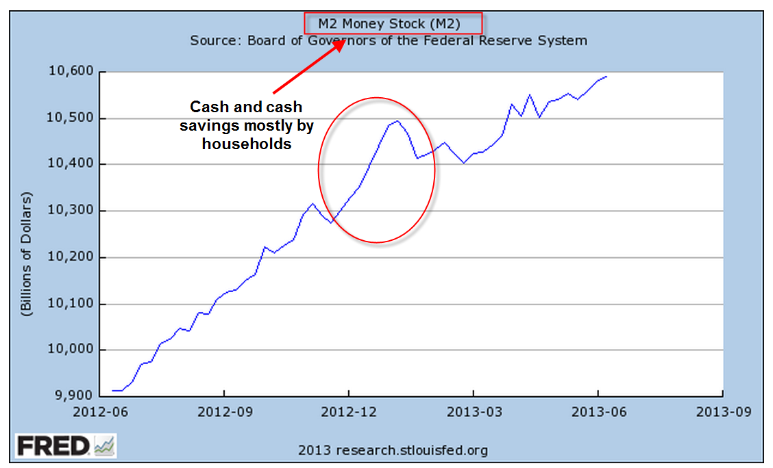
Since the financial crisis, too many investors have adopted a paralyzed strategy, a “deer in the headlight” reaction to the financial crisis that has been hugely unrewarding. Part of this year’s rise in the stock mark can be attributed to individual investors moving cash back into the stock market but I would guess that many of those investors are ready to pull it back out at the first sign of any trouble.  This shows less a confidence in the market but a frustrating lack of alternatives.

Long term bond prices took a significant hit in the middle of the year on fears of an impending rise in interest rates.  Bond prices had simply become too high, driving down the yield, or return, on the investment. Lower bond yields and meager CD and savings rates provided little return for investors, leaving many investors with little choice but to venture back into the stock market.

*************************************
The Coincident Index of Economic Indicators remains level and strong.  A decline in this index below the 1% average growth rate of the population indicates the start of or an impending recession.

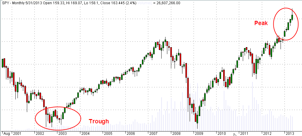
Note the index in 2002 – 2003 as it fell back, never rising above the 1% level.  I have written about this economic faltering before.  Much of the headlines were focused on the lead up to and start of the Iraq war.  The recovery from the recession of 2001 and 9-11 was very sluggish.  Fears that the country was entering a double dip recession similar to that of the early 1980s prompted Congress to pass the Bush tax cuts in 2003.  It was only the increased defense spending of 2003 that offset what would have been a decline in GDP and another recession.

***********************************
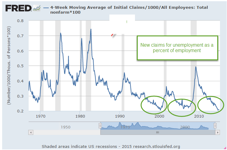
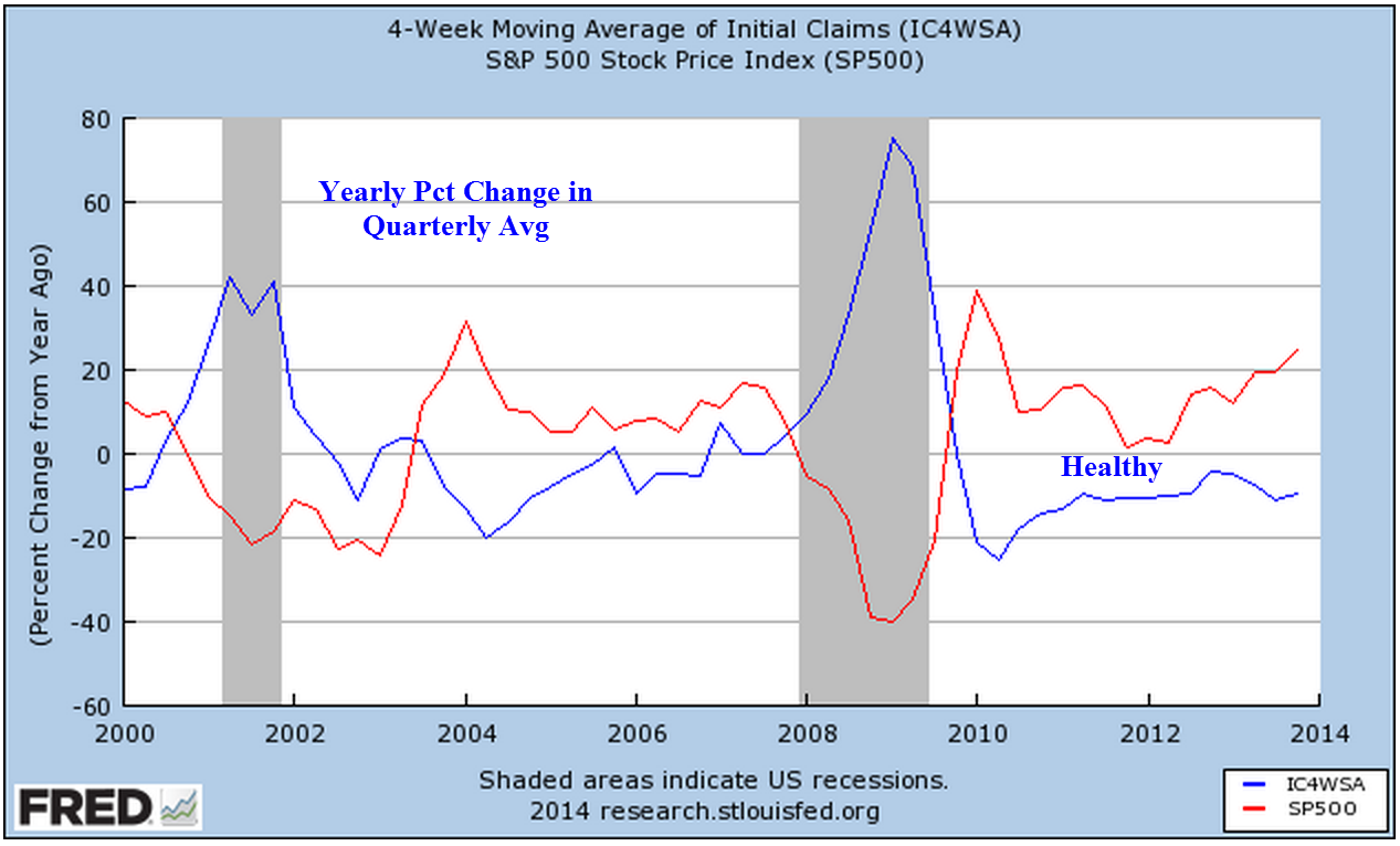
A worrisome rise in new unemployment claims has puzzled some analysts.  Typically, new claims for unemployment decline at the end of the year, particularly in a year such as this one when reports of strong economic growth have been consistent.  Since 2000, rises in claims at the end of the year have been a cautionary note of things to come.  Mid-term investors and traders will be paying attention to this in the weeks to come.

However, the decline this year may be more of a leveling process that has been forming for most of the year.  On a year over year basis, the long term trend is down – which is up, or good.

In March 2013, I wrote “when unemployment claims go up, the stock market goes down … On a quarterly basis, this negative correlation has proved to be a reliable trading signal for the longer term investor.  When the y-o-y percentage change in new unemployment claims crosses above the SP500 change, sell.  When the claims change crosses below the SP500 change, it’s safe to buy. ”  The percent change in SP500 is still floating above the change in unemployment claims.

**********************************
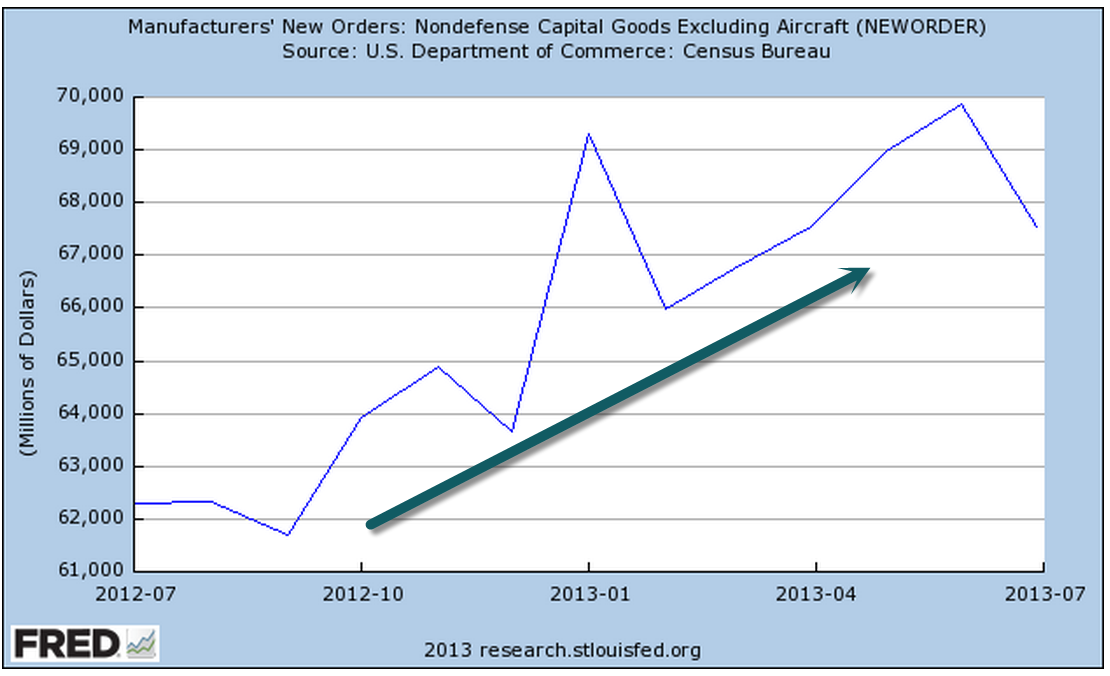
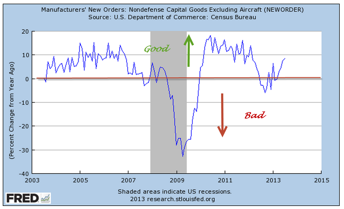
Sales of motor vehicles in November were above even the most optimistic expectations.  The ISM manufacturing index showed a slight decline but is still in strong growth mode and the already robust growth of new orders continues to accelerate.  The manufacturing component of the composite index I have been following since last June is at the same vigorous levels of late 1983 and 2003 when the economy finally breaks free of a previous recession.  I’ll update the chart when the non-manufacturing report is released this coming Monday.

*********************************
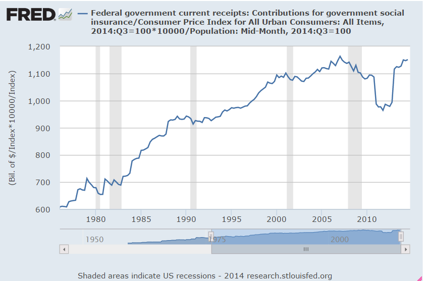
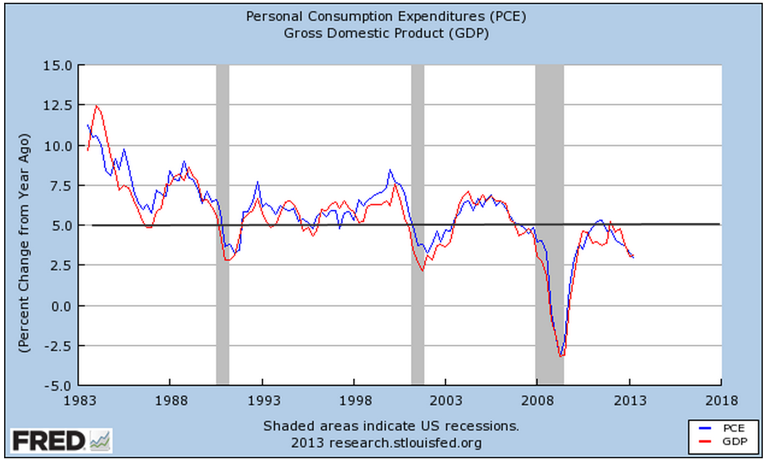
In a healthy economy, the difference between real GDP and Final Sales Less the Growth in Household Debt (Active GDP) stays above 1%, which incidentally is the annual rate of population growth.  As the chart below shows, this difference dropped below 1% in late 2007.  Finally, six long years later, the difference has risen above 1%, indicating a healthy, growing economy.

**********************************
And now a brief look at the year in review.

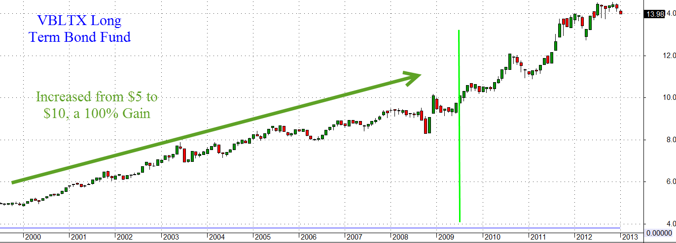
At the end of 2012, the price of long term bonds had declined slightly from the nose bleed levels of the fall but there was more to come.  I wrote “As this three decade long upward trend in bond prices begins to turn, bond prices can fall sharply as investors turn from bonds to stocks and other investments. We are approaching the lows of interest yields on corporate bonds not seen since WW2. Investors are loaning companies money at record low rates and companies are sucking up all that they can while they can. Sounds a lot like home buying in the middle of the last decade, doesn’t it?”

During the past year, long term bonds declined another 10%.  They seem to have formed a base over the past several months.  Intermediate term bonds are less sensitive to interest rate changes so they are the safer bet.  They lost about 6% in price over the past year.  Short term corporate bonds are a good alternative to savings accounts.  They pay about 1% above the average savings account and they usually vary very little in price so that the principal remains stable.

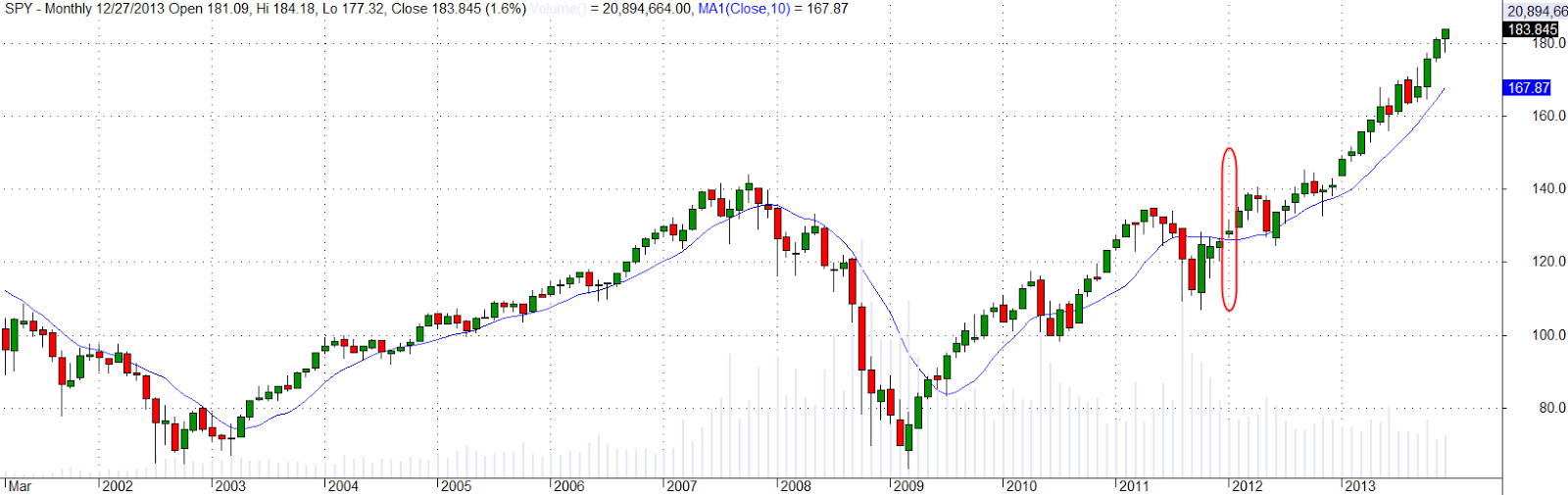
At the end of 2012, I wrote “the underlying fundamentals of the economy give reason for cautious optimism.” A month later, “As the saying goes, ‘The trend is your friend.’ When the current month of the SP500 index is above the ten month average, it’s a good idea to stay in the market.”  In January 2012, the monthly close broke above the 10 month average. This is a variation of the Golden Cross that I wrote about in January and February 2012.

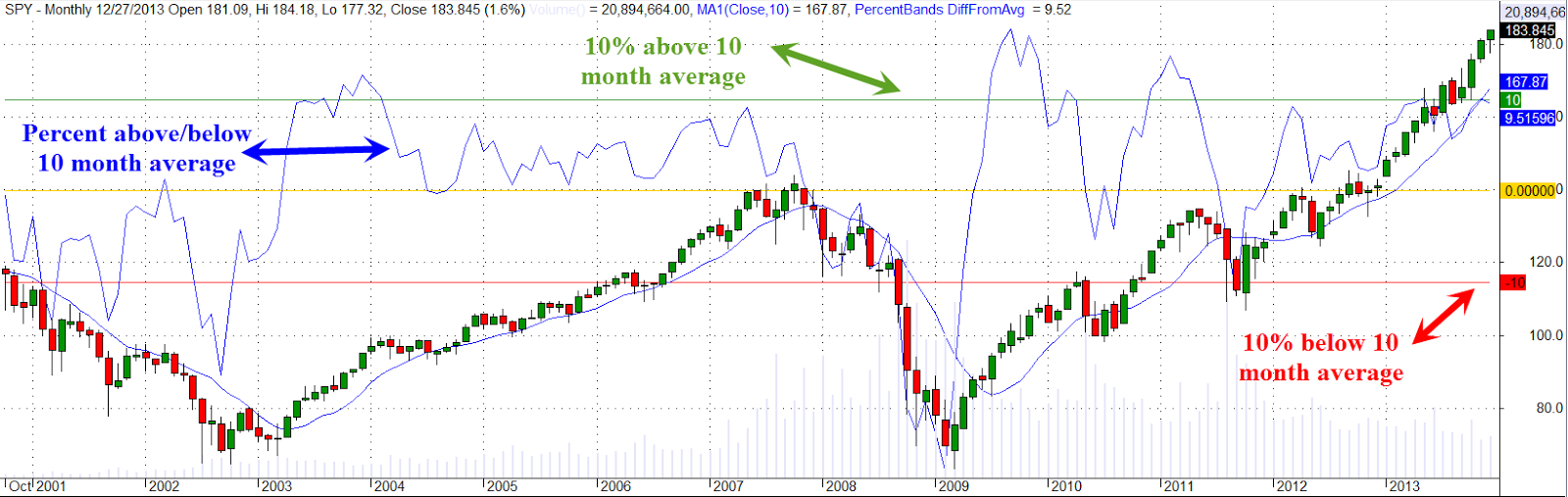
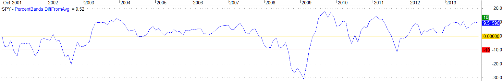
Let’s look at this crossing above and below the 10 month average.    When this month’s close of the SP500 index crosses above the 10 month average of the index, it indicates a clear change in market sentiment.  I have overlayed the percent difference between each month’s close and the ten month average.

As you can see, the close near the end of December is near 10% above the 10 month average.  If the above chart is a bit too much information for you, here is a graph of the percent difference only.

Is the market overheated?  As you can see the market has sustained a robust (or some might call it exuberant) 10% for 6 – 9 months in 2003, 2009, and 2010-2011.  From 1994 to 1999, the market spent a lot of time in the 10% percent range. Some pundits are talking about this market as a bubble but we can see that this market has not penetrated the 10% mark.  At the end of January 2013, the market closed at more than 7% above it’s 10 month average, over the 4 year positive average of 5.6% (the average when the difference is positive).  The market is 20% up since then.

******************************
In March I introduced the “Craigslist Indicator,” the number of work trucks and vans for sale in a local area, as a gauge of the health of the construction industry.  It was a funny little indicator that indicated a growing strength in the construction industry at the beginning of the year.  Now for the amended version of the Craigslist Indicator: when there are a lot of older work trucks and vans advertised for sale on Craigslist, that indicates a robust construction market.

*****************************

On March 24th, 2013 I wrote ” For the past year, the Eurozone has been in or near recession, yet some are hopeful that increased demand in this country and some emerging markets are helping to balance the contractionary influence of decreased demand in the Eurozone. Let’s hope that this surge in the first part of the year does not fade as it did in 2012.”  Instead, emerging markets began to contract and the Eurozone expanded slightly. Investors who bought emerging markets in March 2013 witnessed a more than 10% decline during the summer but the index ended the year at about the same level as nine months ago.

******************************
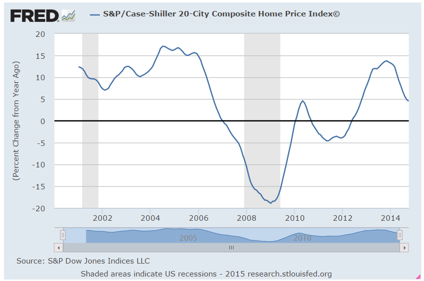
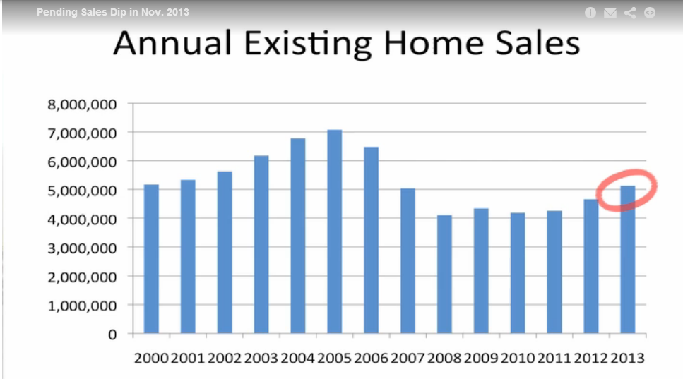
I thought that home prices in the early spring has reached a peak and wrote on March 31st, “The upturn in home prices is still above the trend line growth of disposable income and until personal income can resume or surpass a 3% growth rate, any rise in home prices will be constrained.” The Purchase Only House Price Index (HPIPONM226S) rose steadily throughout the year.
In late summer, I noted the falloff in single family home sales that began in the spring.  But prospective buyers were incentivized to make the deal as interest rates began to climb from their historically low levels.  Home sales surged upward; a lack of inventory in many cities also formed a support base that propped up prices.

A sobering note in September, “Rising home values are good for those who own a home but increasing valuations make it that much more difficult for buyers trying to buy their first home.  People in their twenties and early thirties who are most likely to be first home buyers have been hit hard by the recession.”

*******************************
After a decline in the stock market in June, I wrote “For the long term investor, periods of negative sentiment can be an opportunity to put some cash to work.”  Although I took my own advice, I wished I had acted with more conviction.  Of course, if the market had declined 10%, I would have been patting myself on the back for my cautious stance.  Smiley Face!!

*******************************
In July I noted the rather dramatic decrease in the value of securities held at the nation’s largest banks “Recently rising bond yields have contributed to banks’  operating profit margins but the corresponding value of banks’ bond portfolios has fallen quite dramatically.  This decline in asset value affects bank capital ratios, which makes them less likely to increase their lending … [and] will be an impediment to economic growth.”  The rising stock market and a respite in the decline of bond prices helped stabilize those portfolios in the second half of the year.

********************************
In September, I noted “Despite all the daily and weekly responses to political as well as economic news, the SP500 stock market index essentially rides the horse of corporate profits.”  Profits have more than tripled in the past ten years.  We should stay mindful of that stock price to profit correlation as we look out on the investment horizon.

********************************
From time to time I comment on the venality of our elected representatives.  Although they might appear to be idle rants to some readers, they are a caution.  Politicians make promises to get votes.  People become more dependent on those promises.  Inevitably, the day comes when the promises can not be met – as promised.  Those nearing or in retirement become increasingly dependent on political promises and should leave themselves a cushion – some wiggle room – if possible, when they make income and expense projections.  This Washington Post article on proposed budget cuts to military pensions is a case in point.  As long as “they” come for the other guy, we don’t pay too much attention – until they come for us.  Over the next ten to twenty years, we can expect many small cuts to promised benefits.  The cuts have to be small or target a small sector of the population so that they don’t anger voters too much.  In several blogs, I have shown how a simple recalculation of the Consumer Price Index eats away at the incomes of workers and retirees.  Expect more of these “recalculations” in the future as politicians follow a long standing tradition of making promises to win votes and bargain patronage to gather financial support for their campaigns.

We have the midterm elections to look forward to this year!  OK, calm down. Republicans will be hoping to take the Senate and make President Obama’s life miserable for the following two years.  I am guessing that the political campaigns for some Senate seats will vacuum in more money than the GDP of a lot of small and poor countries.

Investment Allocation and Housing

December 1st, 2013

While cleaning up some old files, I found a 1999 “Getting Going” column by Jonathan Clemens in the Wall St. Journal.  That year was rather turbulent, rocked by Y2K fears that the year 2000 might play havoc with older computers still using a two digit date,  and a intensifying debate about the valuation of stocks.  Looking away from the hot internet IPOs of that year,  Clemens interviewed several professors about the comparatively mundane subject of home ownership.

 “A house is not a conservative investment,” says Chris Mayer, a real-estate professor at the University of Pennsylvania’sWharton School. “Any market where prices can fall 40% in three years is not a safe investment.” 

Remember, this is 1999.  At that time, what 40% decline is he talking about?  It would not be till 2009 or 2010 that house prices tumbled down the hill.  In the past, declines of this magnitude were confined to particular areas of the country where a fundamental shift  in the economy occurred.  The Pittsburgh area of Pennsylvania, the Pueblo area of Colorado and the Detroit area of Michigan come to mind. In the first two examples the collapse of the steel industry had a profound effect on home prices as people moved to other areas to find work.  In case a homeowner thinks “it can’t happen here,” I’m sure many homeowners in Detroit felt the same way during the 1960s when the car industry was at its peak.

“William Reichenstein, an investments professor at Baylor University in Waco, Texas, suggests treating your mortgage as a negative position in bonds.”  

What does this mean?  Let’s say a person has $100K in stock mutual funds, $100K in bond mutual funds, owns a house valued at $200K with $100K still left on the mortgage.  Subtract the remaining balance of the mortgage from the amount in bonds and that leaves $0 invested in bonds.  Why do this?  When we buy a bond we are buying the debt of a company, or some government entity.  A mortgage is a debt we owe.  So, if a person were to pay off the mortgage, trading one debt for another, they would sell their bonds to pay off the mortgage.

Should the house be included in the investment mix?  There is some disagreement on this.  An investment portfolio should include only those assets which a person could access for some cash flow if there was a loss of income or some other need for cash.  An older couple with a 5 BR house who intend to downsize in five years might include a portion of the house in the portfolio mix.

For this example, let’s leave the house out of the investment portfolio to keep it simple. Using this analysis, this hypothetical person has 100% of their assets in stocks, not a 50/50 mix of stocks and bonds.

Now, let’s fast forward ten years from 1999 to 2009.  An index mutual fund of stocks has lost a bit more than 20%.

A long term bond fund has gained about 100%.

[The text below has been revised to reflect the above bond fund chart.  The original text presented numbers for a different bond fund.]

Let’s say the mortgage principal has been paid down $60K over those ten years.  Assuming that no new investments have been made in the ten year period, what is this person’s investment mix now?  The stock portion is worth $80K, the bonds $200K less $40K still owed on the mortgage for a total of $240K, with a net exposure in bonds of $160K.  The person now has 33% (80K / 240K) in stocks and 67% in bonds, a conservative mix.  If we didn’t account for the mortgage as a negative bond, the mix would appear to be 29% (80K / 280K) for stocks and 71% for bonds.  What is the net effect of treating a mortgage balance as a negative bond?  It reduces the appearance of safety in an investment portfolio.

Now let’s imagine that this person is going to retire and collect a monthly Social Security check of $1500.  To get a 15 year annuity paying that monthly amount with a 3% growth rate, a person would have to give an insurance company about $220K (Calculator)   There are a lot of annuity variations and riders but I’ll just keep this simple.  Throughout our working lives our Social Security taxes are essentially buying Treasury bonds that we start cashing out during retirement.

If we were to add $220K to our hypothetical investment mix,  we would have a total of $460K: $80K in stock mutual funds, $200K in bond funds, -$40K still owed on the mortgage, $220K effectively in Treasury bonds that we will withdraw as Social Security payments.  The $80K in stock mutual funds now represents only 17% of our investment portfolio, an extremely conservative risk stance.  If we have a private pension plan, the mix can get even more conservative.

The point of this article was that many people in their 50s and 60s may have too little exposure to stocks if they don’t account for mortgages, pensions and Social Security payments into their allocation calculations.

*****************************

In October 2005, the incoming Chairman of the Federal Reserve, Ben Bernanke, indicated to Congress that he did not think there was a bubble developing in the housing market. (Washington Post Source)

In September 2005 – a month before – the Federal Reserve Bank of New York published a report on the rapid housing price increases of the past decade:

Between 1975 and 1995, real [that is, inflation adjusted] single-family house prices in the United States increased an average of 0.5 percent per year, or 10 percent over the course of two decades. By contrast, from 1995 to 2004, national real house prices grew 3.6 percent per year, a more than seven-fold increase in the annual rate of real appreciation, and totaling nearly 40 percent in one decade. In some individual cities, such as San Francisco and Boston, real home prices grew about 75 percent from 1995 to 2004, almost double the national average. 

Remember, these are real, or inflation adjusted prices.  Now it is easy, in hindsight, to go “ah-ha!” but it should be a lesson to us all that we can not possibly hope to consume all the information needed to mitigate risk.  There is just too much information.  A professional risk manager, Riccardo Rebonato, discusses common flaws in risk assessment in his book “Plight of the Fortune Tellers” (Amazon). Written before the financial crisis, the book is surprisingly prescient.  The ideas are accessible and there is little if any math.

*************************************
On Monday, the National Assn of Realtors released their pending home sales index. These are signed contracts on single family homes, condos, and townhomes. The index has declined for five months but is still slightly above normal (100) at 102.1.  At the height of the housing bubble, this index reached almost 130.  At the trough in 2010, the index was below 80.

This chart was clipped from a video by an economist at NAR (Click on the video link on the right side of the page).  The clear and simple explanation of trends in housing and interest rates is well worth five minutes of your time.  Sales of existing homes have surpassed 2007 levels and are growing.

Demographia surveys housing in m ajor markets around the world and rates their affordability.  Their 2012 report found that major markets in the U.S. are just at the upper range of affordable.  As Canada’s housing valuations have climbed, their affordability has declined and are now less affordable than the U.S.  Britain’s housing is in the severely unaffordable range.

*****************************
Next Friday comes the release of the monthly employment report.  I’ll also cover a few long term trends in manufacturing and construction employment that may surprise you.

Labor and Money Flows

September 1st, 2013

On this Labor Day weekend, I’ll review some things that caught my attention this past week.

The employment picture has shown steady but slow improvement.  The weekly survey of new unemployment claims continues to show downward movement.  In a survey that is about 13 years old, called the JOLTS, the BLS gathers data on Job Openings, Layoffs and Turnovers.  A component of this survey includes the number of employees who have quit their jobs, referred to as the “JOLTS quit rate.” In the aggregate, it indicates a hive intelligence, the estimation of millions of people about the prospects of getting another job.  Decades ago, researchers asked a number of people to estimate the number of jelly beans in a jar.  Each estimate has very small chances of getting close to the actual number, but the average of all estimates was found to be almost exactly the number of jelly beans in the jar.  I don’t know whether this experiment has been replicated but it is interesting.

After recent months of surging new orders for durable goods, July’s report, released Monday, showed signs of caution and a “return to the mean” of a positive upswing this year.

Although this past month’s data was negative, industrial production shows a clear uptrend.

In an analysis released a few months ago, the Federal Reserve examined data from the 2010 triennial (every 3 years) survey of households and estimated that inflation adjusted net worth per household (green line in the graph) has just climbed back to the level it was almost ten years ago.


On the positive side, average net worth is not less than it was ten years ago.  On the negative side for those nearing retirement, it is not more that it was ten years ago.

On Friday, the Personal Consumption and Expenditures (PCE) report showed a 1.4% year over year percent gain, indicating the tepid growth in household spending.  Below I’ve charted the percent gain in PCE vs the percent gain in GDP for the past thirty years.

We are still below the low points of the 1980s, 1990s and early 2000s.  The Federal Reserve is projecting GDP growth of 3 – 3.5% in 2014 but this may be another in a string of rosy forecasts by the Fed, who have repeatedly revised earlier rosy forecasts.  If the Fed were a contractor, it would be out of business due to poor estimating.  A $16 trillion economy is not a kitchen remodel by any means, but it does illustrate how difficult it is for the best minds to make even short term predictions of the economy from the vast amounts of sometimes conflicting data.  Consider then the folly of the Government Accountability Office (GAO), the economic watchdog created by Congress and mandated by Congress to come up with ten year estimates of economic growth and the consequences of existing and proposed legislation.  Those in Congress continue to trot out these fantasy numbers to support or criticize policy and legislation.

Washington continues to vacuum in money and talent from the rest of the country.  Of the richest counties in per capita income in the U.S., the Washington metro area has two of the top three.  The other county in the top three is a stone’s throw from the metro area.  As Washington politicians convince the rest of us that they have the solutions, lobbyists and graduates flock to the concentration of power, jobs, money and influence.
 
Bond yields have increased more than 1% since the spring, meaning that the prices of the bonds themselves have fallen dramatically.  Most of this change has been a reaction to forecasts for stronger growth and a tapering of the Fed’s stimulus program called Quantitative Easing.  Washington is sure to get in the way of stronger growth for the economy as a whole.  Policy out of Washington is designed to promote strong economic growth for Washington.

The market research firm Trim Tabs regularly monitors money flows into and out of the stock and bond markets.  They  reported today that outflows from the stock market in August were half of the record inflows in July.

The blood spilled this year has been in the bond market.  Trim Tabs reports that outflows from bond funds and ETFs have totalled more than $123 billion in the past three months.  Flows into bond funds and ETFs were about $750 billion in 2012, almost a doubling from the $400 billion invested in 2011. (Fed Flow of Funds tables F.120, F.121)

While the prospect of higher rates may have been the trigger that caused a reversal of bond inflows, the underlying current is also an overdue correction of the surge of investment in bonds in 2012.

Households continue to shed debt in one form or another so that total liabilities continue to decline. However, every man, woman and child in this country is carrying, on an inflation adjusted basis, 2-1/2 times the amount of debt they carried thirty years ago.  This level of household liability will continue to put downward pressure on growth.

This next week will kick off with the ISM manufacturing report on Tuesday and finish the week with the monthly employment report.  Year over year percent gains in employment have been steady and guesstimates are for maybe 200,000 net job gains.  150,000 net jobs are needed to keep up with population growth.

The Fed meeting is coming up in mid-September so this employment report will be watched closely to guess the next steps the Fed will take. 

Credit Patterns

July 28, 2013

Economic growth is hampered when credit growth declines.  In 2008, we experienced a sharp decline in confidence and lending that has only now reached the levels before the decline.

When we look at the big picture, we can see that we are now at more sustainable growth trends.

The amount of outstanding commercial and industrial loans is almost at the level last seen in 2008.

A smiliar slow recovery in business loans occurred during the 2001 recession.

Although housing evaluations have been rising, the amount of revolving equity lines of credit (HELOC) continues to decline.  The total outstanding is still high but approaching a more reasonable trendline of growth.

Recently rising bond yields have contributed to banks’  operating profit margins but the corresponding value of banks’ bond portfolios has fallen quite dramatically.

This decline in asset value affects bank capital ratios, which makes them less likely to increase their lending. which will be an impediment to economic growth.

This Wednesday the first estimate of 2nd quarter GDP will be released.  Real GDP growth is expected to be about 1.1%, less than the meager 1.8% growth of the 1st quarter.  Slowing growth may revive interest in bonds.  The recent sell off in bonds has probably been an over reaction incited by fears that the Federal Reserve will reduce its bond buying program dubbed “Quantitative Easing.”  While there are positive signs in the economy, they do not indicate any impending robust growth.

In addition to Wednesday’s release of GDP figures, the payroll firm ADP will show their monthly report of private employment growth, guesstimated to be slightly below the 188,000 gain predicted for June.  The BLS monthly labor report follows on Friday and will be watched closely.  Unemployment has been stuck in the mid-7% range since March and reductions in unemployment have been largely due to people either leaving the work force or taking part time jobs because they could not find full time work.

The Federal Reserve has said that its target for withdrawing its quantitative easing program is an unemployment target of 6.5%, with a caveat that inflation remains tame. A slow economy will naturally reduce inflationary pressures and improvements in the labor market are slowing as well.  In short, the Fed is likely to continue its monetary support for another year at least.

For a month now, the stock market has risen steadily in small increments, making up the losses that began in the third week of May.  Volume typically declines during summer months but this year’s volume of trading in SPY, the ETF that tracks the SP500 index, is 20% lower than this same time last year.  This week, we may see a market hesitation before the release of both the GDP and labor reports.

The Great Moderation

June 30th, 2013

Economists cite a number of factors to account for the growth during the 1980s and 1990s, a period some call the “Great Moderation” because it is marked by more moderate policies by politicians and central bankers.  Causes or trends include less regulation, lower taxes, lower inflation than the 1970s, the rise of emerging economies,  and a more consistent rules based monetary policy by the Federal Reserve.  Often underappreciated, but significant, was the huge increase in consumer credit. Household spending accounts for 2/3rds of the economy.  A new generation, the boomers, emerging fully into adulthood in the early ’80s, welcomed the broader availability of credit.  Like their parents, the boomers took on the burden and responsibility of owning a home, the largest portion of a household’s debt load, but unlike the previous generation, the boomers sucked up as much credit as they could get for cars, clothes, vacations, home furnishings and the growing array of electronic devices.

When we look at the non-mortgage portion of household debt, the rate of growth is more restrained – a mere 80% increase in per capita real dollars.

The parents of the boomer generation, dubbed by newscaster Tom Brokaw as the “Greatest Generation”,  had been habitual savers.  By 1980, the personal savings rate was about 10% of disposable income.  By the middle of that decade, the Greatest Generation began retiring and withdrawing some of that savings.  Their children, the boomers, did not have a similar sense of frugality.

Rapid advances in technology led to the introduction of new electronic toys for adults.  Credit cards, once reserved for the well to do, became ubiquitous.  Consumers parted with their money more painlessly when charging purchases.  Financing terms for automobiles became more generous,  allowing more people to purchase new cars, which became increasingly expensive as regulators mandated more safety controls.

After thirty years of gorging on credit, households threw up.  The past six years could be called the “Great Diet” or the “Great Purge” to get over the three decade credit binge.

We can expect rather lackluster growth for several more years as households continue to shed those ungainly pounds debts.  Not only are households shedding debt but also certain kinds of assets. In 2009, the Federal Reserve reported that households and non-profit corporations owned $400 billion in mortgage securities like Fannie Mae and Freddie Mac.  In the first quarter of 2013, the total was $10 billion.  (Table of household assets and liabilities)

Households continue to keep ever higher balances in low yielding savings accounts and money market funds, indicating the high degree of caution. The big jump in deposits was probably due to higher dividends and bonuses paid in the last quarter of 2012 to avoid higher taxes in 2013.

For the past two weeks, global markets shuddered at the prospect of the Federal Reserve easing up on their quantitative easing program of buying government bonds.  Some have proclaimed that it is the end of the thirty year bull market in bonds, causing many retail investors to pull money out of bonds.  In several speeches this past week, Reserve Board members have reassured the public that quantitative easing will be here for several years.

As we have seen, households still shoulder a lot of debt weight, making it unlikely that either this economy or interest rates will experience a surge upward in the next several years.  An aging and more cautious population together with a declining participation rate in the work force indicates that another “Great Moderation” is upon us.  The previous moderation was one of political policy.  This moderation is led by consumers.  We can expect – yes, moderate, or lackluster – growth over the coming years.  The positive tradeoff for this subdued growth is the probability that the underlying business cycle of growth surges and corrective declines in economic activity will be subdued as well.

Summer Sale

June 23rd, 2013

It would be a mistake for the casual investor to think that the decline in the market this week was due entirely to Fed chairman Ben Bernanke’s comments regarding future Fed policy.  There was little that was not anticipated.  The Fed will continue to follow a rules based approach to its quantitative easing program, scaling back its purchases of government securities if employment improves or inflation increases above the Fed’s target of 2%.  Bernanke also reiterated that the Fed would increase its purchases if employment does not improve and inflation remains subdued.  So why the drop?

Shortly after the conclusion of each Fed meeting, Bernanke holds a press conference, where he issues a ten minute or so summary of the meeting and issues discussed.  He then takes about twenty questions.  At the start of this past Wednesday’s press conference at 2:30 PM EDT, the market was neutral as it had been all morning.  The Fed chairman was more specific about the anticipated timeline of the wind down of quantitative easing if the economy continued to improve.   Although he was essentially repeating himself, the voicing of a specific and concrete timeline evidently jolted some sleeping bulls who surmised that the party was over; in the final hour of trading the SP500 fell a bit more than 1% in the final hour.  For many traders, it was time to take profits from the eight month run up in prices.  “Quadruple witching”, a quarterly phenomenon that occurs when stock and commodity options and futures expire, was approaching.  The few days before this event usually see a spike in volume as traders resolve their options and futures bets.

With much of the Eurozone in a mild recession and slow growth in emerging markets, the rest of the world perked up their ears as the central banker of the largest economy envisioned an easing of monetary stimulus sometime in 2014.

Overnight (Wednesday/Thursday) came the news that the Shanghai interbank rate had shot up from about 4% to 13%, a rate so high that it threatened to seize up the flow of money between Chinese banks.  This bit of bad news from the second largest economy added additional downward pressure on world markets.  For some time, analysts covering China have been warning about the amount of poorly performing loans at China’s biggest banks.  The spike in interbank rates, prompted by the Chinese government, was an official warning to Chinese banks to be more cautious in their lending practices.

On Thursday morning came the news that jobless claims had increased, adding more downward pressure.  The SP500 opened up another 1% lower that morning and dropped a further 1.5% during the trading day. This classic “one-two” punch knocked the market down about 4%.  European markets fell about 5%, while emerging markets endured a 7.5% drop in two days.

In the past four weeks, there has been a decided shift in market sentiment.  When the market is bullish, it tends to shrug off minor bad news.  As it turns toward a bearish stance, the market reacts negatively to news that just a few months ago it largely ignored.

Over the past two months, long term bonds have declined 10% and more.  Here is a popular Vanguard long term bond ETF that has declined 12% since early May.

For the long term investor, periods of negative sentiment can be an opportunity to put some cash to work.

Stocks vs Bonds

June 2nd, 2013

As the market makes new highs this past month, I am reading articles and seeing charts on asset allocation that reminded me of those I saw in 2000.  Here is a chart that appeared in the WSJ this weekend.

Mutual Funds typically report their performance over several time periods, usually 1, 3, 5, and 10 year periods.  This spring, as the SP500 index continue to peak, a ten year lookback window begins near a trough in the index in the spring of 2003.

Why did the WSJ writer pick 25 year and 35 year time periods as a comparison?  We can only guess but it just so happens that the starting points of these two lookback periods were also troughs in stock prices.  Why not pick 20 and 30 year time periods? Let’s look at the 25 year period which starts in April 1988.

What if the writer had used a 20 year lookback?  They would have started in April 1993, when the stock market was 72% higher.  I don’t want to take the time to calculate the difference in returns, including dividends, between the different strategies shown in the chart, but the reader can imagine that the difference would be significant.

Why use a 35 year lookback?  Why not a 30 year lookback?  In 1978, the SP500 index was again pulling out of a trough in prices after a slow slide in values during 1977.

Had the WSJ writer picked a 30 year window starting in April 1983, the stock market index was – again – 72% higher than in April 1978.  Again, we can imagine that the comparison of strategies would be significantly different.

Being aware of these peaks and troughs can help us evaluate past performance of various investment allocations.  Consider an example of a 10 year comparison of the SP500 vs a bond index fund like Vanguard’s VBMFX

The SP500 index shows the better return but, if we know that spring of 2003 was a trough in this index, we can view such a comparison with some skepticism.  A five year comparison tells a different story.

Now we are comparing performance starting with a downslide in the index, when the SP500 had fallen about 11% from its peak.  It is also close to the 3 year moving average of the SP500 index.

Based on a five year window and the fact that our starting point was a 3 year average in the SP500, we might conclude that our portfolio should contain mostly bonds.  Who needs the aggravation of the volatility in the stock index when we can make the same return with a boring bond index?

In a 3 year time frame, stocks have clearly outperformed bonds.

Our starting point of this 3 year window also happens to be the 3 year average of the SP500 index.  Not only that, it is just  a bit above the midpoint between the 2007 index peak and the trough in the spring of 2009.  We couldn’t ask for a more reliable starting point to make our comparison.

So we have a second reliable starting point but the conclusion we draw is significantly different from the conclusion we drew in the 5 year comparison.  Let’s look closer at this stronger performance of the SP500 vs a bond index.

Half of the better 3 year performance of stocks has come in just the last 6 months after the Federal Reserve announced their open QE program of buying government bonds until the unemployment index reaches a target of 6.5%.  The recent upsurge in stocks has “goosed” the comparison numbers upwards in favor of stocks.

Our conclusion is that historical performance numbers presented by mutual funds or an investment advisor cannot be taken at face value.  It is important to understand the starting point of the historical comparison, which can have a significant effect on the numbers.