Rollercoaster

January 11, 2015

Price movement continued to be volatile in this second week of the year.  Despite all the price gyration, the SP500 is down only 1% since the first of the year.  On Monday, light crude oil broke below the $50 price barrier, helping to usher in a rush to safety, namely U.S. government debt.  As the prices of long term Treasuries climb upwards, who is buying this Federal debt?  As the chart below shows, foreigners already hold the majority of Federal Debt.

As the dollar continues to strengthen, institutional investors around the world buy Federal Debt to enhance the return on their savings. Let’s say a European investor bought $132 of Treasury debt on September 1, 2014 for €100. Now that same investor cashed in that U.S. Treasury bill this past Friday.  What does the investor get back?  €111.46, without any accrued interest or fees included. In a little over 3 months, they have made almost 11-1/2% return, an annual rate of more than 40%.

On the other hand, the “carry trade” is getting squeezed.  The carry trade involves borrowing money in a country with a low interest rate, or borrowing low, and buying debt in another country with a higher interest rate, or loaning high.  This is a great deal – easy money – IF the currency of the country where an investor borrowed the money doesn’t start rising in value as the U.S. dollar has done recently. The problem is particularly acute in emerging countries which have higher interest rates to attract capital.

To keep the example simple, let’s use the euro again.  On September 1st, a European investor bought €100 of  French BTFs paying 5%.  Because interest rates are so low in the U.S., the  European investor was able to borrow the money in the U.S. for 1/2%, making 4.5% for doing nothing.  The investor borrowed $131.30, converted it to €100 and bought the BTFs.

This past Friday, the U.S. bank calls the investor’s loan so the investor cashes in her €100 BTF and gets only $118.42 at the current exchange rate.  They are short $12.88, an annualized loss of almost 36%.  What makes this simple scenario even more dangerous is that, in the real world, the investor has often leveraged their money, multiplying the losses.

The problem becomes particularly acute for companies headquartered in an emerging market (EM) country but which have a U.S. subsidiary.  The subsidiary borrows money at a low interest rate in the U.S., much lower than the prevailing rate in the EM country, then converts those dollars to the currency of the EM country to fund expansion.  If the EM currency loses value against the dollar, the company finds it increasing difficult to make payments on their loan because each time they convert their EM currency to U.S. dollars, the EM currency buys fewer dollars.  This is another kind of squeeze that may cause the bank to call the loan, or escalate the loan to a higher interest rate, creating even more financial pressure on the company.

This is the first time in fifteen years that the U.S. dollar has gained in strength against all major currencies.

***********************

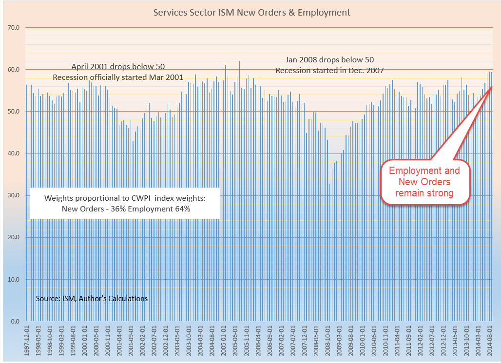
Purchasing Manager’s Index 

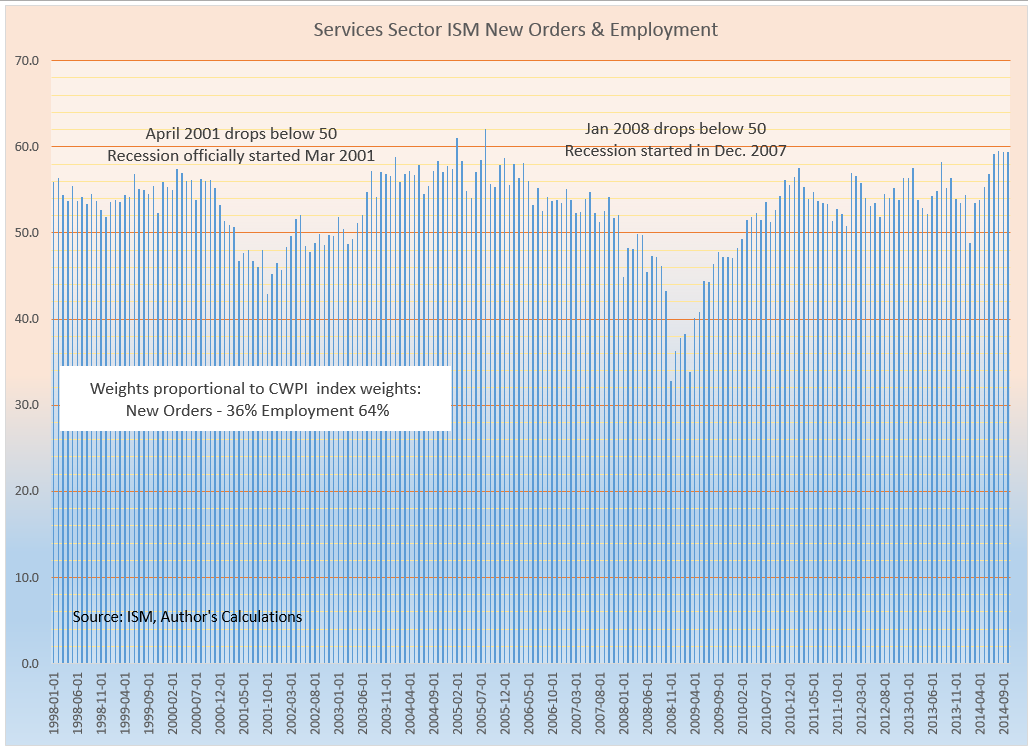
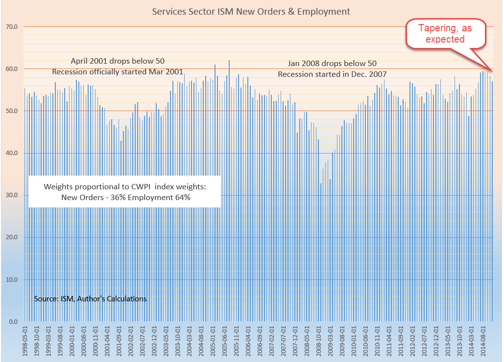
As expected a few months ago, a composite of employment and new orders in the services sector continued to moderate in December.  In September, these two key factors of production were at the highest levels in 17 years, so some decline was anticipated toward the end of the year.

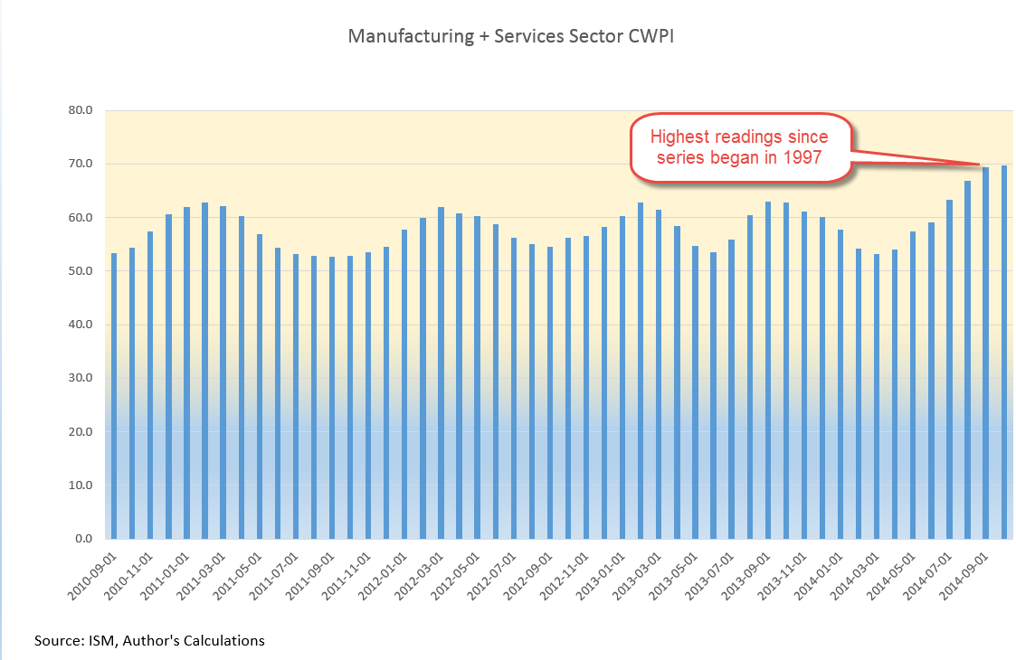
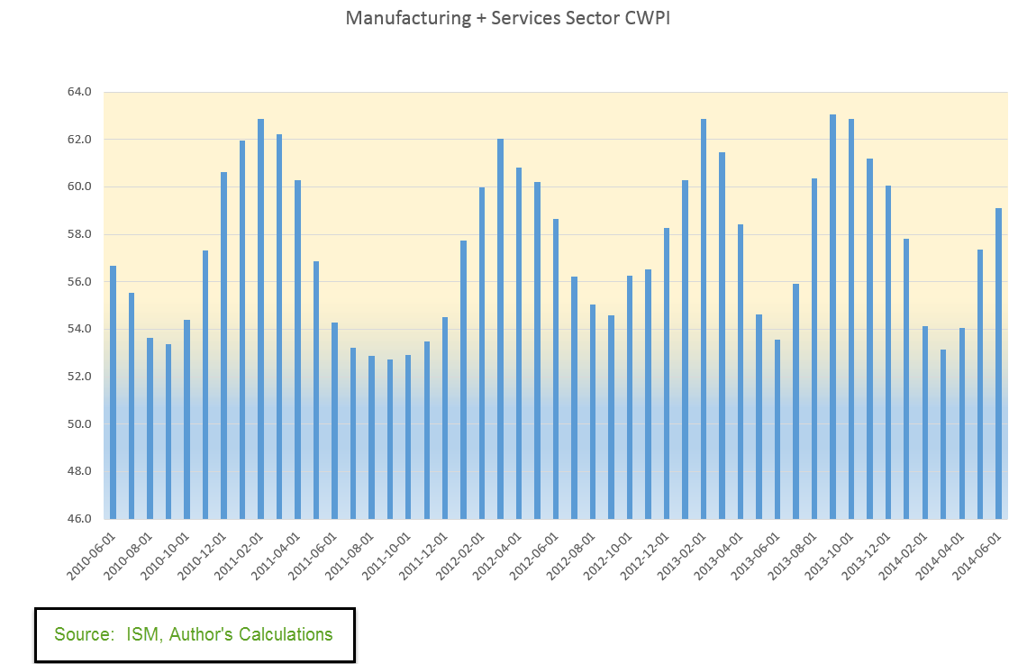
The CWPI, a composite of manufacturing and services sector activity in the country, continues to run strong, although it has also moderated from the higher peak set in October 2014.  The wave like pattern of economic activity is getting stronger over the past several years.  The peaks are coming closer together and now the strength of activity has quickened.

Despite these strong economic indicators, investors are worrying again (see October blog)  that the rest of the global economy is faltering. Why investors showed less concern about the global economy in November and December remains a puzzle. To longer term investors, the market seems to have the attention span – and frenetic activity – of a three year old.

************************

Employment

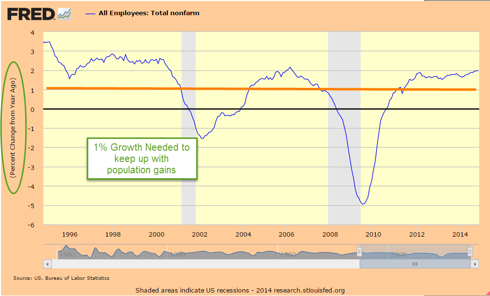
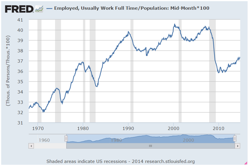
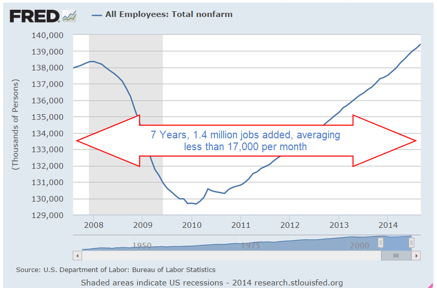
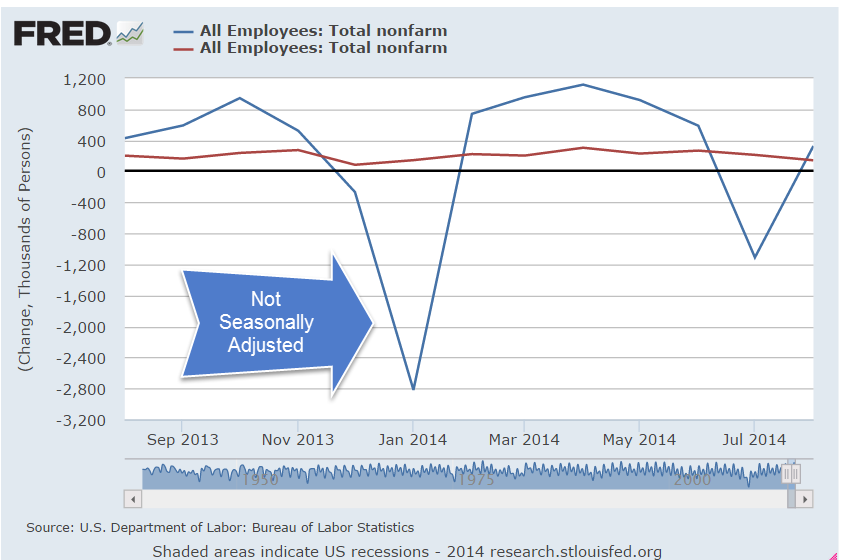
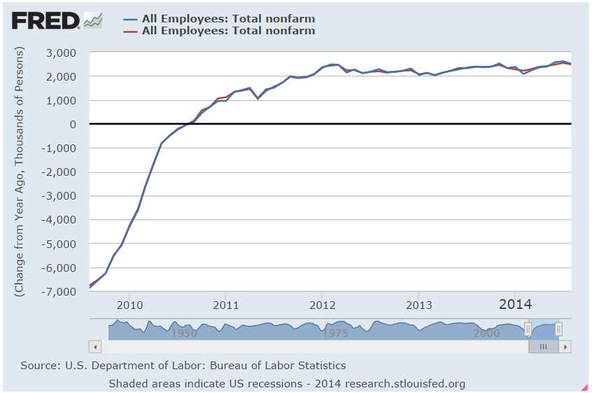
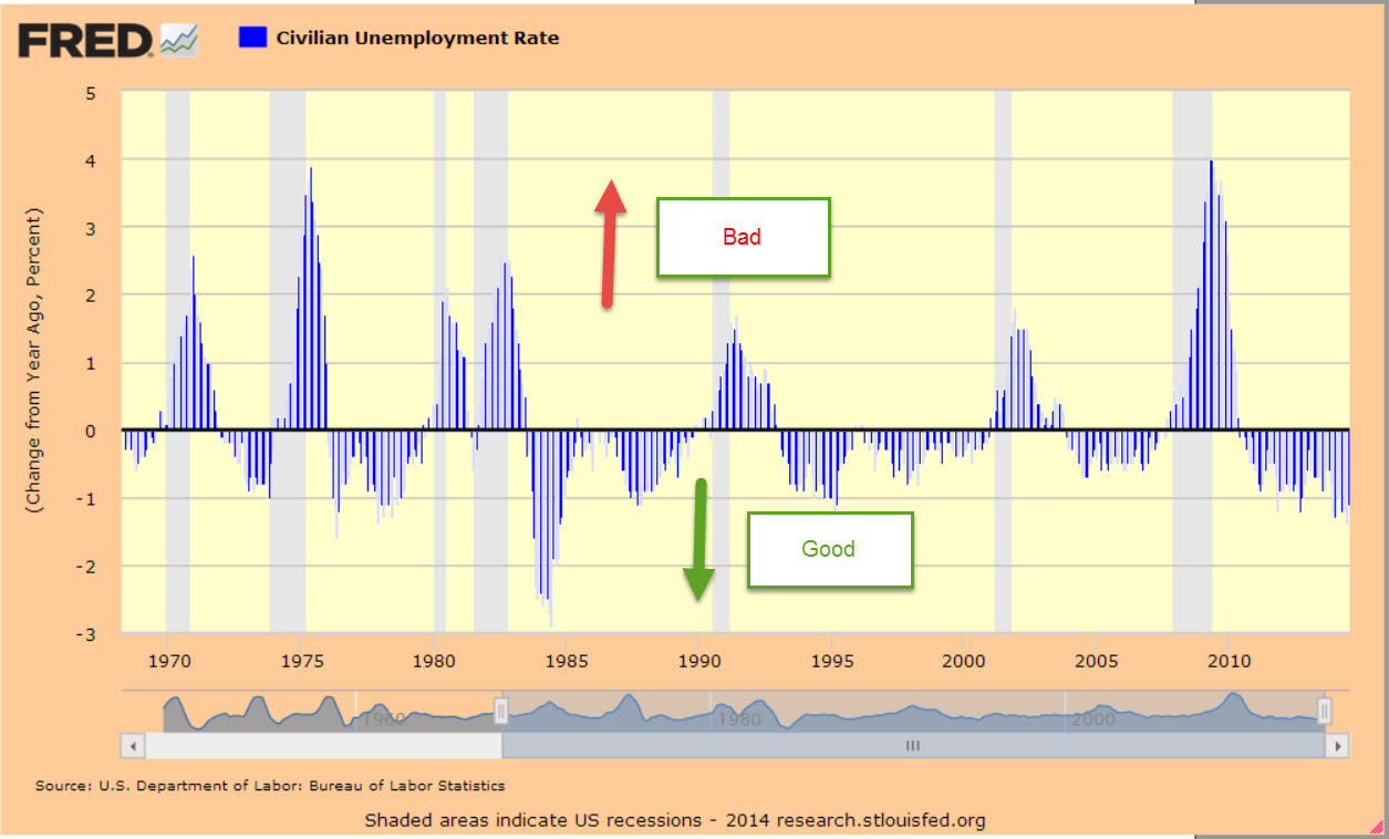
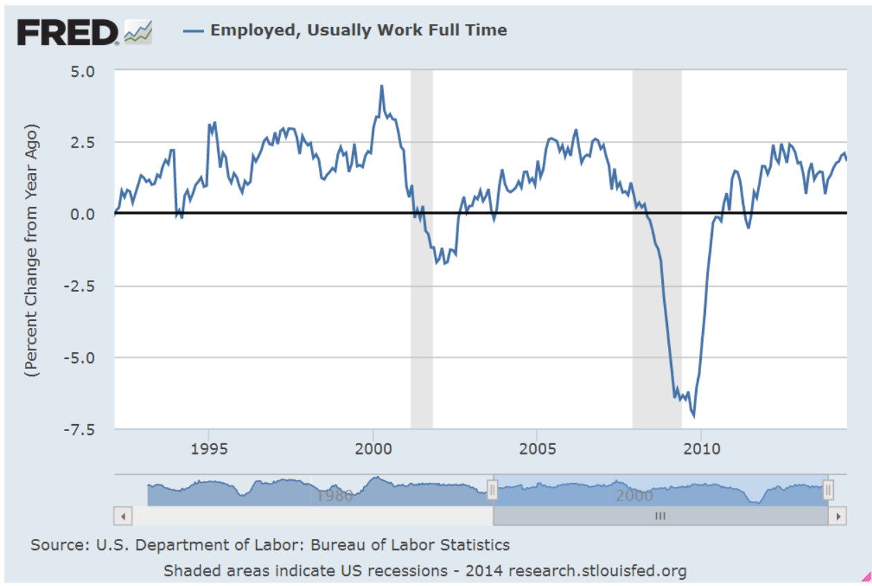
In December, employment rose 2.1% year over year, almost besting the high set in March 2006 for yearly growth.

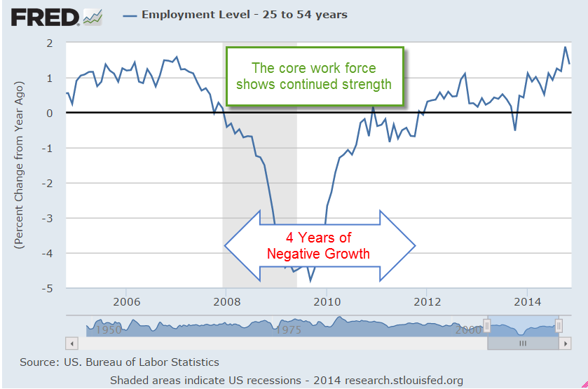
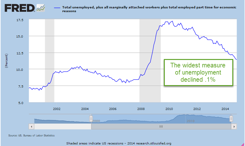
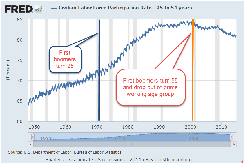
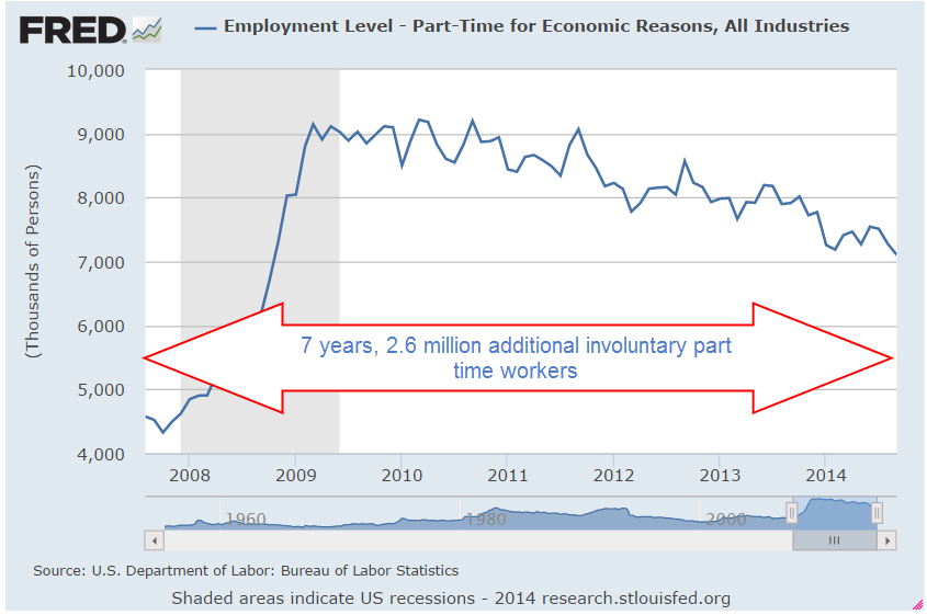
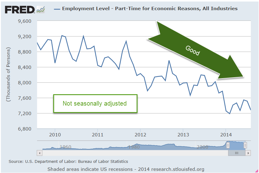
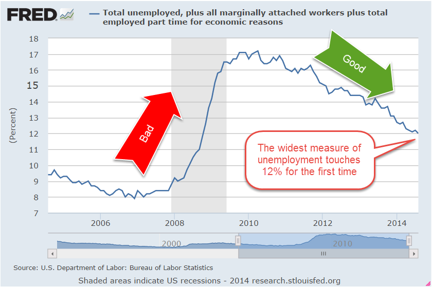
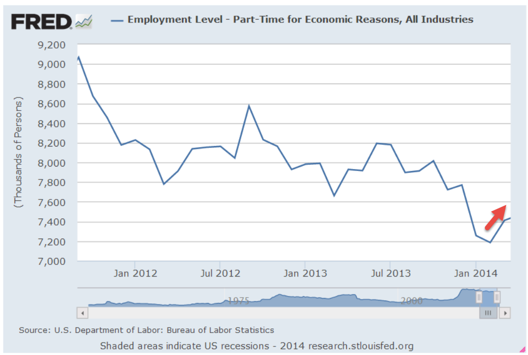
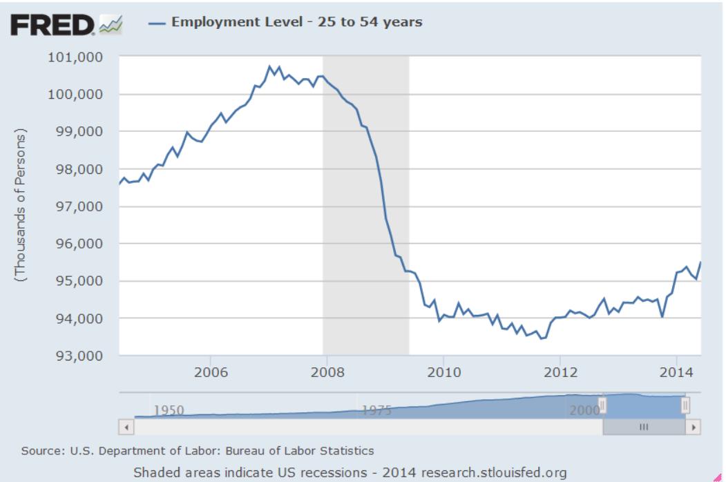
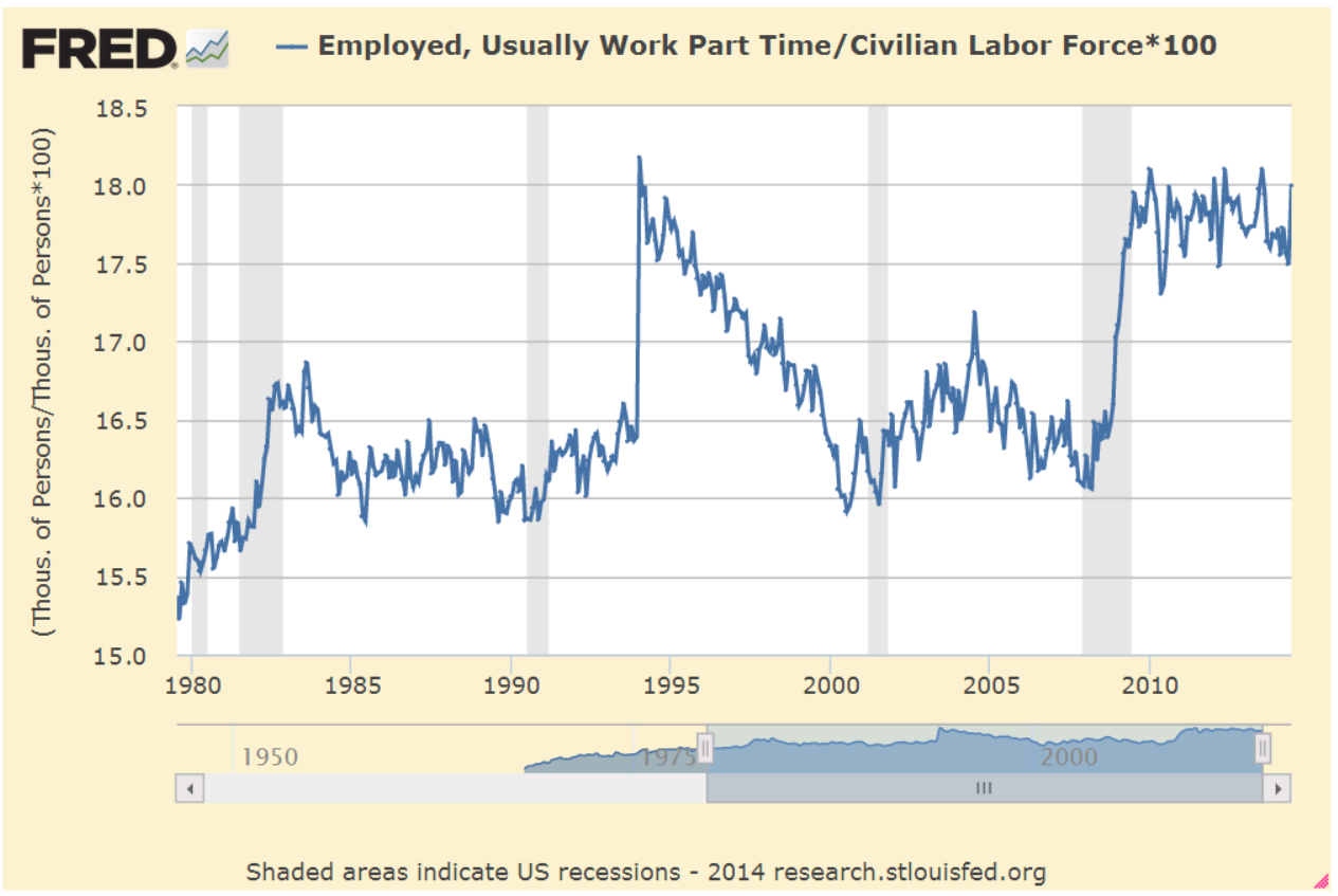
There were several positives in this report.  Job gains for October and November were revised up 50,000 total.  The core work force, those aged 25 – 54, continued a steady rise. The number of people employed at part time jobs because they couldn’t find full time work fell again in December by 60,000 and is down 13% over the past year.  However, there are still 50% more involuntary part-timers than during the 2000s.

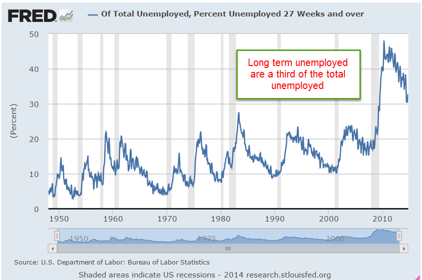
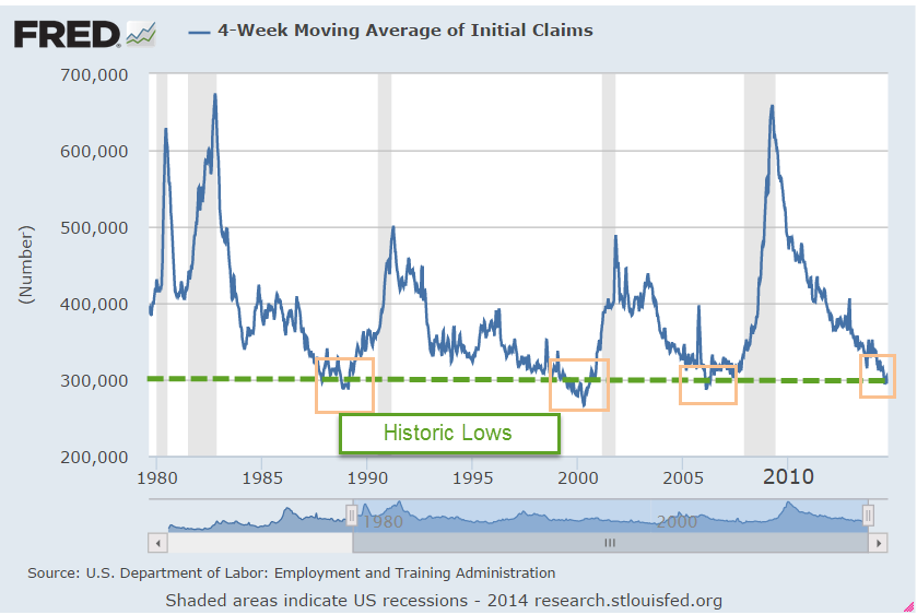
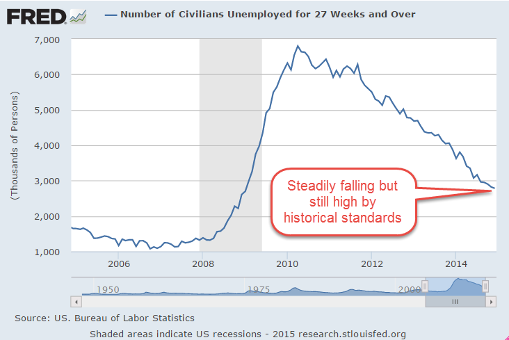
The number of long term unemployed people has fallen 28% in the past year but – that word “but” rears its ugly head again – are still high.

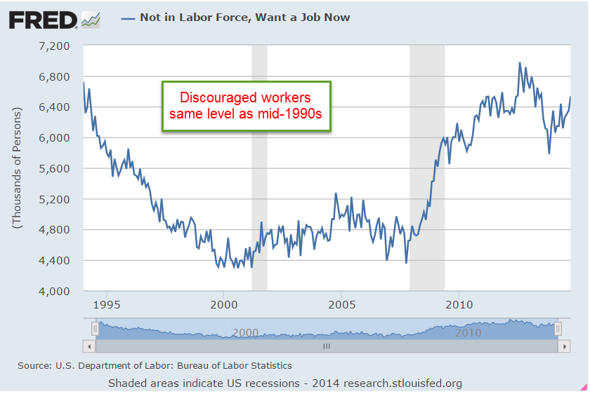
Investors tended to focus on the negatives in this month’s report.  The number of discouraged workers, those who are available for work but haven’t looked in the past month, was up 42,000.

As a percent of the labor force, the long term unemployed and discouraged are still at historically high levels – more than five years after the official end of the recession.

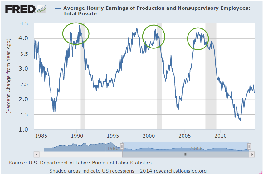
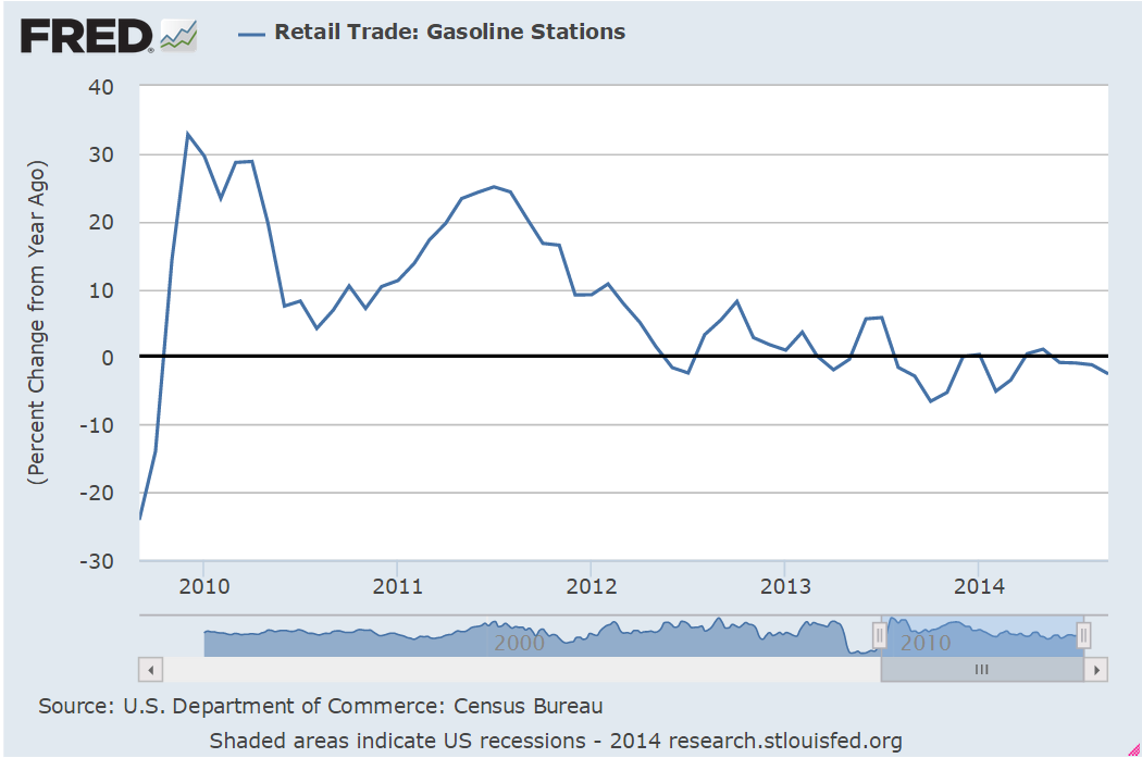
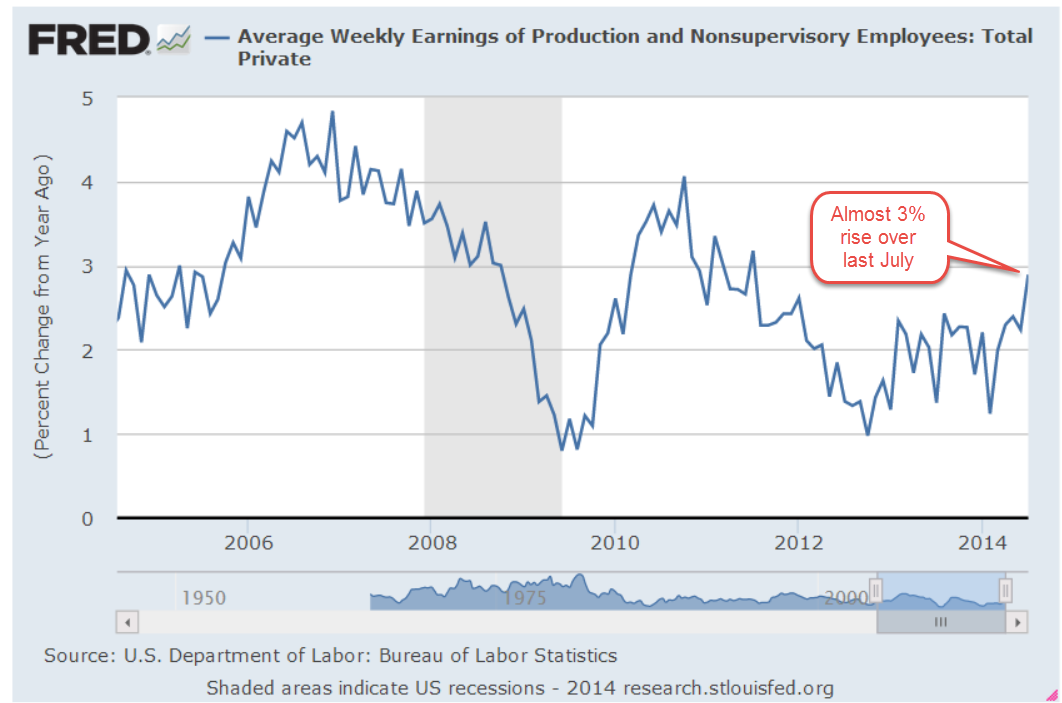
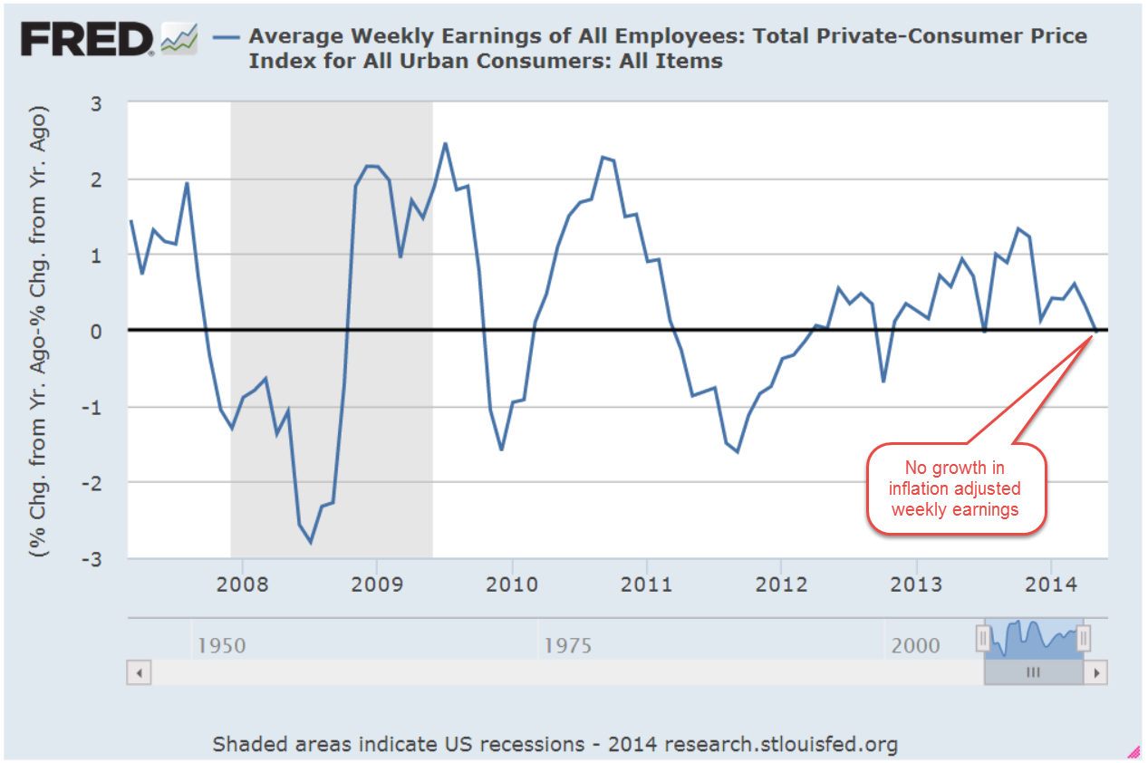
Hourly wages declined by .05 to $24.57 but the influx of seasonal and part time jobs at the holidays and year end may have had some impact.  Last month’s slight increase in hourly wages sparked hope that employees might be gaining some pricing power, indicating an underlying strong demand from employers.  This month’s data suggests that lower gasoline prices will have to substitute for wage growth in the near term.

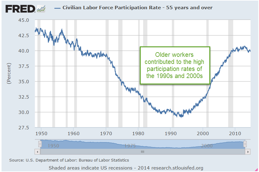
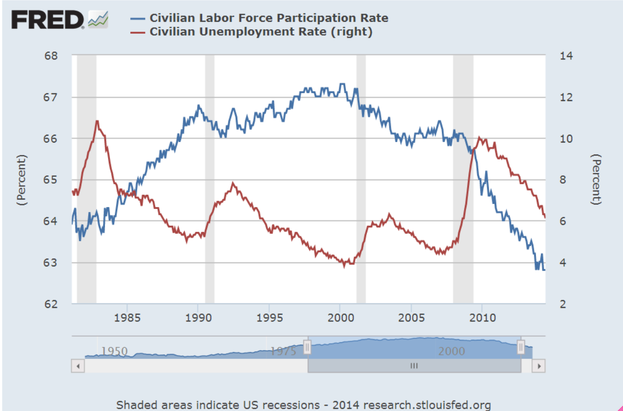
The Labor Force Participation rate edged down .2 and seems to be stuck in a range just under 63% for the past year.  If the labor market were really growing strongly, we would expect to see some upward movement as more people tried to enter or re-enter the job market.

************************

Social Security Calculator

Last year the Wall St. Journal reviewed several social security claiming calculators.  Social Security (SSA) has some very complex rules, particularly for married couples.  Remember that this is a system designed by politicians and the Washington bureaucracy, the same people who, after 9-11, designed the multi-colored terror threat warning system that seemed permanently stuck on yellow, or elevated threat.
 
Given the complexity of the Social Security rules, noted economist Lawrence Kotlikoff heads a team that designed an online calculator  to help people maximize their benefit.  The program has a fee of $40 and looks very easy to use.  An 11 minute video demonstrates using the tool for a married couple born in 1958 and 1952.  Curl up on the couch and get out the popcorn.

The mutual fund giant Fidelity has a good discussion of various claiming options for married couples.  The third example is rather interesting.  The younger person in a married couple files early and receives a reduced benefit. The older person files and suspends his own benefits at full retirement age (FRA) but takes a spousal benefit based on the fact that his wife has already retired.  Here’s the kicker: his spousal benefit is based on what her benefit would have been at FRA, not the reduced benefit she receives because she retired early.

*************************

Allocation

We learned about allocation while playing Monopoly.  It is better to put up a few houses on both the Green and Purple property groups than put all of our money into hotels on the pricey Green group only.

Vanguard has a questionnaire to help investors determine an appropriate allocation mix of stocks, bonds and cash.  You don’t need to be a Vanguard customer to answer the questionnaire.

*************************

Final Word

The price of oil is unusually low.  The U.S. dollar is unusually strong.  Interest rates have been unusually low for several years.  Central banks around the world have provided an unusual level of support for their economies.  A confluence of unusualness, a new word, leads to greater price swings.  Market volatility (VIX) has been low – below 20 – for most of the past two years and this relative calm tends to bring more people into the market, helping to lift stock prices.  We may see a return to higher volatility levels similar to early 2012 and late 2011.

Gangbusters!

December 7, 2014

On Monday, George intended to put the $50K from the CD into the bond market. He couldn’t decide between a long term bond index like Vanguard’s BLV or TLT, the ETF that tracked 10 year Treasury bonds. Both the bond and stock markets opened lower in the morning which confused him and he did nothing. Gallup released their monthly survey of consumer spending for November, showing a respectable gain of more than 4% over last November.

Tuesday’s report of auto sales in November was strong.  Total vehicle sales topped 17 million on an annualized basis. Auto manufacturers reported particularly strong sales over the Thanksgiving holiday.  SUVs were big sellers and that was a double plus for auto companies because those vehicles had larger profit margins.  The American car buyer has long had a short memory.  Six months of falling gas prices prompted many to abandon their economical cars and wrap themselves in a big bubba vehicle.

Construction spending was up 1.1% from the previous month and 3.3% above last October.  The economies of Europe may have slipped into neutral or recession but the U.S. economy was chugging along.  The upbeat reports gave the stock market a minor boost but there was little selling of Treasuries, indicating a growing split in sentiment among investors.  George decided to put his and Mabel’s CD money into TLT.

On Wednesday, the Centers for Medicare and Medicaid Services released their annual report on health care costs.  Spending had increased only 3.6% in 2013, the lowest increase since 1960, and the fifth year in a row that spending had grown less than 4%.  Out of pocket expenses had risen from $293 billion in 2007 to $339 billion in 2013, a 16% increase over six years.  Before the recession, George could remember years when spending rose almost that much in a single year.  CMS reported that consumers’ out-of-pocket spending was only 3.2% of charges, less than the 5.9% of charges in 2007.

CMS published a historical table that caused George to raise both eyebrows.  In 1960, Americans spent $125 ($967 in 2012 dollars) per person on health care. In 2012, that figure had grown eight-fold to $7533 per person.  Administrative and public health programs added another 15% to those costs.  In 2013, the total cost per person was over $9500 for a whopping national total of $2.9 trillion spent on health care, almost 18% of GDP.

While families were shelling out more for health care, companies were grabbing a larger share of the economic pie.  As a percent of GDP corporate profits had been trending upward since 1990.

The private payroll processor ADP reported private job gains of 208,000, slightly below expectations but still above the 200,000 mark considered a healthy job market. Later that day came the announcement that a Staten Island grand jury decided that there would be no indictment in the death of Eric Garner.  Caught on video, five or six officers had surrounded the man to arrest him for selling bootleg loose cigarettes.  One of the officers put a choke hold on the unarmed Garner, restricting his breathing till he died of asphyxiation.

Later that day, four Denver bicycle cops were escorting a parade of students protesting the grand jury decision in Ferguson.  Acting as a buffer between the students and traffic on the busy street east of the Capitol, the officers were struck by a Mercedes as it ran through an intersection.  The Mercedes dragged one of the officers about thirty yards and that officer was taken to the hospital in critical condition.  On the evening news, George and Mabel learned that the driver of the Mercedes might have been having a seizure when he hit the officers.

Late Thursday morning, George was focused on several economic reports.  Since 2010, the polling firm Gallup had conducted a simple employment survey, called P2P, that counted the number of people who had worked for money in the past week or had looked for work in the past week.  Gallup reported the lowest unemployment rate, 6.2%, since the poll began.  New jobless claims were one again just under 300,000, indicating that the previous week’s 314,000 might have been an anomaly.  The 4 week average of new claims was still below 300,000.

Friday morning the reporters dusted off their sports dictionaries as they searched for words to describe the monthly labor report from the BLS.  Blockbuster.  Gangbusters. Blowout numbers. Spectacular.  Amazing.  George poured another cup of coffee. Yes, 321,000 new jobs sounded great!!! Too great. George got out his magnifying glass, put on his Sherlock cap and went hunting.  First of all, ADP had reported 208,000 private job gains.  The BLS report included new government jobs which the ADP did not include.  So back out the 7000 new government jobs to get private job gains of 314,000 according to the BLS.  Paging Dr. George, number surgeon.  He took out his skeptical scalpel. Take the average of the two estimates, which was 314 +  208 = 522, divided by 2 = 261.  Add back in the 7000 government jobs and probably the more accurate figure was close to 270,000 – 280,000.  September’s job gains had been revised up 20,000 by both ADP and the BLS. The BLS also revised the job gains of October,  getting closer to the averaging method that George used. Sacre bleu!  Averaging really works!  George was a big believer in averages.

Anyway, the employment report was strong, just not as fantastic as it first appeared. Average monthly job gains for the past year had been about 230 – 240,000.  George picked up his magnifying glass.  Hmmm, he said.  Retail job gains were 50,000, far above the 22,000 average of the past year.  At least 20,000 of those job gains were temporary seasonal gains.  Let’s be generous and start with 280,000 jobs. 280 – 20 = 260.  Now job gains were approaching the average of the past year.

Still, the yearly growth in employment was climbing toward 2%, slowly but surely getting stronger.

Professional and business service jobs had been a leading sector for the past few years and were especially strong this month at 86,000, way above the average gains of 50 – 55,000.  George raised a skeptical eyebrow.  A closer look showed that the strong gains were particularly strong in bookkeeping and accounting.  Take out 20,000 temporary tax jobs, George thought, and now his count was down to 240,000.  Boy, this was quickly becoming an average employment report.

Yearly gains in hourly earnings for the average worker were just under 2.2%, just barely ahead of inflation. For all workers, the gains were 2.1%.

George put away his magnifying glass and put on his rosy glasses.  The average hourly work week had increased .1 hour over the past month, a good sign.  However, that was also the yearly gain.  Not so good.  George cleaned his rosy glasses.  The gains had been fairly broad and the core work force aged 25 – 54 had increased to nearly 96 million.

The construction and manufacturing sectors reported strong gains.  Although the headline unemployment rate remained the same at 5.8%, this rate was more than 1% below last year’s rate, a sign of a relatively healthy labor market.

A wider measure of unemployment, the U-6 rate, had declined .1% but was still above the rates in the mid-2000s.  George needed a better pair of rosy glasses.

George checked to see if the Federal Reserve had updated their Labor Market Conditions Index but that would probably come next week.  The market had risen a few tenths of a percent since the high of two weeks ago.  According to a Fact Set report, earnings growth for the fourth quarter had been revised down from 8.3% to only 3.4%.  After rising up almost 14% since the mid-October trough, the SP500 had stalled despite a number of positive reports.  Treasury bonds had lost a few percent in price since mid-October but had stayed relatively strong, indicating some skepticism toward any further stock gains.  The stock market seemed to be treading water ahead of the December 11th deadline for Congress to pass a spending bill.  Despite promises that there would be no government shutdown this time, investors might be a bit less confident in the dependability of promises from the Republican leadership.

A Long Term Plan

November 16, 2014

“Yaaaaay!” Charlie erupted as he kicked the pile of leaves in the backyard. Rusted orange, dried blood crimson and mustard yellow flew up into the air.  Rake in hand, George smiled at his grandson’s exuberance. “Hey, champ, let’s get these leaves in the bag.”  The little arms gathered up the colored leaves and swung to the trash can which was about the same height as the four year old boy.  Charlie threw the leaves up over the lip of the trash can.  Very few leaves made it into the can. Charlie tilted the black plastic can toward him so that he could look in the can. “Look, Ganpa!” he exclaimed, proudly showing the inside and the few leaves that had made it into the can.  “The kid’s a politician,” George remarked to his son Robbie sitting on the back deck. “Get’s very little accomplished with a lot of fanfare.”

Robbie held up his phone. “Let me get a shot of the two of you.”  George picked up Charlie and held him over the trash barrel.  Charlie clasped him around the neck and Robbie snapped the picture.  George set the child down and the boy once again gathered up a clump of leaves and threw them up into the air.  Robbie took another picture of his son.  George walked over to the deck.  “Let me see.”  Robbie showed him the two pictures then looked at the picture of his son tossing up the leaves.  He handed the phone to his dad.  “Looks like a scatterplot, doesn’t it?” Robbie asked. George looked.  “Wow, what have you been working on?  Most people don’t see a scatterplot in a cloud of leaves.” A scatterplot is a number of data observations plotted on a graph.

“Still working on pattern recognition for drones,” Robbie said, a bit of tiredness in his voice.  “A lot of tough problems to crack.”  George nodded toward Charlie. “I can remember when you were this age,” George said, a fondness in his voice. Robbie went on, “Charlie – any four year old – has better visual processing that the most sophisticated algorithms we write. The brain scientists plot the paths in our brains but we still sit around the lab wondering what is it that our brains are doing when we interpret the world.  Well, we just keep kicking at this mule…” His voice drifted as Charlie came over to them, leaves clenched in his little fists.  He slumped on Robbie’s knees.  “You need to rake more leaves, Ganpa,” he whined.  George looked up and saw that Charlie had leveled the pile of leaves.  “Ok, champ, let’s rake more leaves.”

Mabel opened the rear screen door.  “I need a potato peeling person!” she called out.  Robbie stood up.  “I’ll get it,” Robbie said, “you rake.”

As he raked, George thought back to that time when Robbie was the same age Charlie was.  At that time, thirty years had seemed like a lifetime because it was.  He and Mabel had been in their thirties.  George remembered some  meetings with their accountant at the time. She had given them the talk, one that she probably gave to other young families. “You need to keep some things in mind for your kids, and for your retirement.  I know it seems like a long time away now but your little boy will be in college before you know it.”  The accountant was only a few years older than they were but talked like a Solon.  George had supposed that the profession encouraged that kind of long term thinking.  Heck, his time horizon was about five years and this woman was stretching their imagination out twenty, thirty and forty years. “The choices you make now will limit or expand your choices in the future.”

Almost thirty years later, George and Mabel had done well by following her advice over the years.  George wanted to thank her but she had moved her business to Oregon or Washington and they had lost touch.  They had not bought the really big house although they had sometimes wished they had more room, especially when the kids were teenagers.  They had treated the two houses they had owned as a place to live, not as an investment vehicle or a store of wealth to borrow from.  The mild downturn in the residential market in the early 1990s had not worried them.  When the prices of homes crashed in 2007 and 2008, they lost little sleep because the mortgage was paid off.  George did take a hit on his 401K though.  He was close to retirement as the market tanked and both of them worried a lot through that 2008 – 2009 winter.

In the late 1980s, George had opted in for what was then a fairly new idea, a 401K plan, at work.  These were termed “defined contribution” plans.  The employee, not the employer, took the risk and the responsibilities for the investment allocations in the plan.  The employer made its contribution to the plan and had no long term liabilities for the results that the investments did or didn’t make.

When Mabel returned to teaching in the mid 1990s, she had taken a conventional defined benefit pension plan, the only one that the school offered.  In early 1999, as the Nasdaq climbed to nosebleed valuations, George had eased up on the stock allocation in his 401K.  He didn’t know a whole lot about investing, only that stocks were riskier than bonds.  As the market continued to climb, he sometimes regretted his decision but stuck with it as a matter of common sense. By the end of 2000, as stock prices continued to fall, he was glad he had been more conservative.  In late October 2014, the Nasdaq 100 had finally climbed above the level it reached in 1999, 15 years earlier.

They enjoyed a wonderful Sunday dinner with Robbie, his wife Gail, and their grandson Charlie.  Robbie asked about Emily, his sister, but no they hadn’t heard from her in almost a year.  Two kids grow up in the same house.  One of them is stable, has a good career, and a wonderful family.  The other leads a troubled life, and is consumed by some inner demon.  Emily was not a fit conversation for a dinner table so the talk moved onto other topics.  Robbie, Gail and Charlie drove back to Colorado Springs that evening.  There was a front moving down from Canada or Alaska so they declined the offer to stay in the guest room for the night.

There wasn’t a lot of economic news scheduled for the week so George was not expecting any strong moves in the market.  Much of the earnings season had come and gone.  According to FactSet  almost 80% of companies had reported above consensus estimate of earnings.  A more disturbing sign: three times as many companies had issued negative guidance for fourth quarter earnings as those that had indicated a more positive outlook.

The big news for the week was the Rosetta spacecraft.  Launched ten years earlier, it had rendezvoused with a comet 300 million away on its journey from the far reaches of the solar system to the sun.  As if that wasn’t spectacular enough, the spacecraft then launched a washing machine sized landing vehicle to sit down on the comet as it sped through space.  Talk about long term planning.

On Thursday, the spot price of a barrel of crude oil dropped below $75.  The Energy Information Agency (EIA) announced that the average price of a gallon of gasoline had fallen further to $2.94, the second week below $3.   Several analysts pegged the price range of $65 – $70 as a “make or break” benchmark for many fracking operations.  If oil were to stay down at that level for any length of time, many new drilling plans would be put on hold.  Operations at existing wells might be cut back.  The strong dollar meant that countries who were net exporters of oil would be paid in dollars, which could be traded for more of their own currency.  For these countries, the strong dollar was helping offset the impact of lowered prices.

On Thursday, the BLS released the September report of job openings and turnover, or JOLTS.  The number of employees quitting their jobs had risen to a recovery high of 2%.  Workers who were not confident of finding another job did not quit their current job.  Job quitters acted as a canary in a coal mine, where a relatively small part of an ecosystem or economy indicated the health of the entire system.  A rate of 2% or higher indicated a healthy confidence in the employment grapevine.

On Friday, George had lunch with a few former colleagues.  Four old guys sitting at a booth, drinking too much coffee. As usual, the discussion was lively.  Each of them had a take on the elections just past but the conversation got a bit heated when Stan said that there were just too many people who didn’t want to work.  Who was going to pay for all these people?  Who was going to pay for all the government programs?  He had just read a report from Pew Research that summarized the changing trends in the labor force participation rate and the sometimes contentious debates about those changes.  The participation rate was the number of people working or looking for work as a percentage of the adult population, the civilian non-institutional population, as it was called.  A 90 year old person could still work and was counted as part of that population of potential workers.

The core work force, those aged 25-54, showed a slightly declining participation.  The first boomers had grown out of this age group at the turn of the century.

George’s opinion, one echoed by the Congressional Budget Office, was that much of the reduction in the participation rate was due to changing demographics.  Since the mid-1990s, women, particularly white women, had had a historically high participation rate.

Some workers of earlier generations who had not needed a college education to earn a middle class wage found themselves less desirable in this more technological work environment.  During the recession, employers shed many workers with long term health problems.  As the economy improved employers were reluctant to hire these job seekers who may have had a good work ethic but possessed no above average skills or education.   Some applied for disability, or retired early if they could, or simply gave up trying.

Those with college level education and higher were more likely to be working.  The downtrend in the participation rate for both groups had started during the Clinton years, long before the Bush presidency, the 2008 recession or Obama’s presidency.

Full time workers as a percent of the total population were about the same level as the mid-1980s, when the economy was in a growth phase.  The 1990s and 2000s had been marked by unsustainable bubbles – the dot com boom and the housing debacle.

Older workers contributed to the high participation rates of the 1990s and 2000s.  A lot of people came to regard these abnormally high participation rates as normal.  They weren’t, George argued.

Sure, people are living longer, George argued, but the number of older workers can’t keep rising indefinitely.  Since the early 1990s, older workers had risen by 20 million, from 12% of the work force to 24% of the work force.  They were competing with younger workers for jobs.

27% of the entire population was older than 55.  Most of that population was past working age yet older workers made up 24% of the work force.

Workers who might have retired in decades past were continuing to work, clogging up the labor pipeline.

Stan thought the economy had still not recovered and was worried about the next recession.  Who’s gonna pay for all these people, he wondered again.  George reminded him that average weekly hours of all private workers – most of the work force – was now at the same level as before the recession.

The Civilian Labor Force was higher now than before the recession started.  The growth rate was lower but still growing.

But George agreed that there were persistent problems.  A third of those unemployed had been out of work for more than a half year.

Real weekly earnings were stagnant, neither growing or declining.

There were still a lot of people who were not counted in the labor force because they were not actively looking for work.  They wanted jobs but had given up.  As bad as it is now, George reminded Stan, discouraged job seekers are at the same level as they were in the mid-1990s.  Did you even notice back then?  George asked.  Stan admitted he hadn’t.

“A lot of us weren’t paying attention,” George told the group seated at the booth.  “Sure, it got bad sometimes, but we figured we would get through it.  This last recession was bad, bad, bad and there is a lot more information available now.  We can see how bad it was five years ago and there’s plenty more information to worry over as we look to the future.”

“So, you’re optimistic?” Stan challenged.  “Yeh, I am,” George replied. “Thirty years ago my accountant told me that by the time we retired, politicians would have to do one of three things:  increase taxes, cut benefits, or increase the retirement age.  She told Mabel and I that politicians would probably do a little of all three to spread the pain out and avoid getting thrown out of office.  I was doubtful.  How could she know what was going to happen so far in the future?  ‘It’s just math,’ she told us. ‘The largest generation of people is going to start turning 65 in twenty-five years and the system is not designed for it.  They’re gonna get sick and who’s gonna pay for it?  You think the little that you pay into Medicare is going to cover that?’  I look back now at her predictions.  They’ve raised the retirement age.  Check. The low inflation rate is helping to reduce the growth in Social Security benefits.  A half-check.  Medicare costs are growing at two to three times the rate of inflation.  They haven’t raised taxes yet but it’s coming.”

Stan said sardonically, “And you call yourself an optimist.”  George laughed.  “I guess I’m an optimist because she got Mabel and I planning for all of this a long time ago.  When they raised the retirement age, we weren’t surprised.  When they cut Social Security benefits in the future, we won’t be surprised.  When they raise taxes, we won’t be surprised.”

“Is this lady still your accountant?  She sounds pretty smart.” Stan asked.  “No,” George replied. “I think she and her husband moved to Oregon or Washington.  They wrote business and investment software but they gave up trying to defend their software from copying.  This was in the late 1980s and early 1990s.  Even their own clients were copying their software and giving it to their friends. ‘Smaller companies like ours just don’t have the time or resources to protect against theft,’ she told us.  ‘Eventually we’ll go to work as consultants for the larger companies.’  And several years later, that’s what they did.”

The waitress brought the check.  Normally they would split it four ways but Stan picked it up and handed it to George.  “Shouldn’t the optimist pay?”  George laughed.  “This one time,” he said, “but on one condition.  You all have to agree with me.  Isn’t that how they do it in politics?”  They all laughed, grunting as they straightened up after sitting so long.

Adjusting the Carburetor

November 9, 2014

About two thirds of companies in the SP500 had reported earnings for the third quarter. George guessed that positive earnings surprises were somewhat above the normal 70% but as former Presidential contender Herman Cain said, “I don’t have facts to back that up.”  Checking his guess, George went to Fact Set which provides a weekly update summary of earnings reports.  Positive earnings surprises were the highest percentage in over four years. On the other hand, Fact Set was reporting that the forward price earnings ratio of the SP500 was above the 5 and 10 year average.  Einstein famously quipped that the most powerful force in the universe was compound interest.  He might have mentioned an equally powerful force – reversion to the mean.

George updated his spreadsheet with data from Robert Shiller, the Yale economist who had devised the CAPE ratio, an inflation adjusted Price Earnings ratio for the SP500.  When the CAPE was higher than average, as it had been the past two years, price gains over the following five years were likely to be low or negative.  George had added a spreadsheet column to measure the annual percent gain in stock prices five years in the future, then plotted these five year gains against the CAPE ratio.  In the long run of several years, the above average gains in stock prices of the past few years were likely to drift lower or turn negative, bringing their 5 year return to the post-WW2 historical mean of 7%.

But in the post-WW2 period, the stock market had almost always gained in the year after a mid-term election.   It’s like a junction on a hiking trail with many signs and no mileage, George thought.

Monday’s report on auto and truck sales was almost exactly in the middle of the range of expectations.  Promotional sales in August before the introduction of 2015 models had propelled sales upwards in August. Sales in September and October had stayed on trend, a sales curve that was flattening.

Manufacturing data from ISM was strong and continuing to rise, but the market seemed to be in pause mode a day before the elections.  “One more day!” Mabel exclaimed. “We’re being bombarded with political ads.” George reflected on that for a second. “I don’t think I’ve actually seen one ad,” he said.  “We buzz through them when we’re watching a program.”  “Well, sometimes I like to watch the local news live or the weather channel,” Mabel responded.  “It’s become impossible to watch anything live on TV.”  George wondered how many millions would be spent on this election.  How many voters were like he and Mabel, paying little if any attention?  Mabel was a straight ticket voter.  It took her less than ten minutes to vote.  Amendments to the Colorado Constitution – no. “Don’t you even read them?” George had once asked her.  “Nope, they’re all sponsored by special interests,” she had replied.  “What about the marijuana amendment two years ago?” George had asked. “Well, I did vote yes on that one,” Mabel had conceded.  George spent hours researching candidate bios and their positions on the issues.  He would sometimes bring up a name of an independent candidate or a Libertarian candidate to Mabel.  “Why waste your time?” Mabel had asked.  “Whether we like it or not, we’ve got a two party system in this country.  Pick one and vote.  No Independent or Libertarian candidate is going to win.” “Yeh, what about Ross Perot in ’92?” George had asked.  “Cost Bush the election,” Mabel had responded. “No, it didn’t.  Perot took about as many votes from Clinton as he did from Bush,” George had argued.  Where had he read that?  Probably Wikipedia.  “Fine,” Mabel had countered with that tone of voice meaning end of argument.

As they watched election results on Tuesday, George commented that he had been wrong.  “No!” Mabel exclaimed, her hands raised in supplication to the fates.  “Let me write this down,” she said. “Hecklers, always the hecklers,” George shook his head in a mock display of discouragement. “No, really.  I thought the Republicans would gain the Senate but just barely.  Gardner is cleaning Udall’s clock.  Look at Mia Love in Utah.  Methinks there’s a change in the wind, oh forsooth.”

Colorado was a toss-up.  As they turned in for the night, one channel had declared the Republican gubernatorial candidate, Bob Beauprez, as the winner in the race.  In the state senate and house, the Democrats held a slim majority that could be overturned but the races were too close to call.  George expected a bump up in the market the next day unless ADP, the private payroll processor, had a disappointing report of private job gains.

Wednesday morning they woke to the news that incumbent Colorado governor John Hickenlooper had squeaked out a win but his rival had still not conceded.  State senate and house races were still undecided and there might be recounts through November. “If this were a baseball or football game, this would be exciting.” George’s banter had little effect with Mabel who was in a rather sour mood. “Look,” he added, the Dems will have a chance to take back the Senate in 2016.  The Republicans will have six or seven Senate seats up for grabs by the Democrats.  It’s the math of Senate elections.”

In addition to gaining the Senate, Republicans had extended their control of the House.  George turned to the ADP report of private job gains – 230,000.  The market had popped up about 1/2% at the open, showing a curious restraint after the previous night’s Republican sweep.  One of their CDs would be due in a few weeks but George knew this was not a good time to bring up the subject of moving some of that really safe money into something else.  Their son Robbie, his wife Gail and their grandson Charlie would be coming over this weekend and that would help brighten up the mood in the house.

The price of West Texas Intermediate crude oil crossed below the $80 mark.  The game was on to control the world market for oil.  Fracking in the U.S. had increased supply, reducing net imports of oil by the U.S.  However, the cost per barrel using fracking methods is more expensive than conventional drilling.  The only way that the Saudis could strengthen their dominance of the market was to drive the price down to a point where fracking was no longer profitable, putting pressure on these suppliers.  At a price below $80, plans to start new wells might be put on hold.  At a sustained price below $80, some suppliers with higher drilling costs might shut down or reduce their output.  Russia, Venezuela and Mexico depended on a higher oil price to fund their governments and social programs.  The lower revenues from oil were exerting a lot of political pressure within these countries.

ISM released their monthly report on the service sectors.  George added the new data to his spreadsheet. He had expected a decline from September’s peak, but the composite of manufacturing and non-manufacturing was as strong as September.

Employment and New Orders were two key factors in the services sector.  For the fourth month in a row, the readings pushed the 60 level, the boundary between strong growth and robust growth.  There had only been two times in 2005 when readings had been this strong.

 On Friday, the BLS released their monthly report of employment gains.  Although net job gains were slightly below expectations, there were gains in most industries, a healthy sign.  As usual, George averaged the BLS estimate and ADP’s estimate.  Subtract the 5000 new jobs in government from the 214,000 reported by the BLS to get private job gains of 209,000.  Average that with the 230,000 jobs estimated by ADP to get 220,000, then add back in the 5000 government jobs. A strong report in a string of strong reports.

George had heard a number of explanations for the swing toward the Republicans. The economy was growing.  Why had voters handed such a decisive hand to the Republicans?  It was a repudiation of Obama’s failed policies.  George noticed that Mabel had not eaten all her nacho chips from the night before. There are rules so he asked politely if he could finish them.  Chipotle’s chips were the best. No, they were Democrats focused on tactics rather than ideas.  No, it was a resounding affirmation of conservative principles by the Amuhrican people. No, it was a throw the bums out election.  No, it was a frustrated electorate that is sick of Washington gridlock and a do-nothing Congress.  No, it was shifting sentiments among age groups and demographic groups. Voters over 60 were a greater percentage of voters in this election while voters under 30 were a smaller percentage.  Asian and Hispanic voters had voted Democratic but with less commanding majorities.  Men swung Republican more than women swung Democratic. Post-election analysis sometimes reminded George of post-Super Bowl analysis.  There was one chart that encapsulated a big problem that Democrats had.  Part-timers couldn’t find full-time jobs.

Each of those 3 million extra involuntary part-timers were counted as one job, regardless of the hours.  A little more than 1 million jobs had been created since the peak of employment in 2007.  Job growth, in short, had been paltry.  A good indicator of job growth was Social Security tax revenue collected each year. In 2006, near the height of the housing boom, the Federal Government had collected $809 billion in Social Security taxes (Treasury data), a 27% increase over the amount collected in 2000, at the height of the dot com boom, just before George Bush took office.  In 2008, the year before Obama took office, the government collect $674 billion.  Six years into Obama’s tenure as President, the government would collect about $755 billion in 2014, a modest increase of 12%.  It was true, Obama had been handed an extremely dysfunctional financial system and a global economy in a death dive.  

Strong wage growth had preceded the past three recessions.  Since this past recession, wage growth had fallen and stayed persistently low, causing discontent among frustrated voters.  Many workers were barely keeping up with inflation.

Voters were like the shade tree mechanics of George’s youth.  To adjust a carburetor, turn the screw this way or that way, trying to find the position where the engine idle sounded the smoothest.  It was a negotiation of sorts between air and gas.  Every two years, voters turned the political adjustment screw and waited to see if it made a difference.

Wild Ride

October 19, 2014

On Monday, Mabel met for lunch with several friends, both active and retired teachers, to celebrate a new inductee into the Million Mistake Club.  Mabel had once explained it to George, “It started a few decades ago when Mr. Densmore – he taught trigonometry at the school – commented one day in the break room that he had passed the two million mark.  He was probably in his late fifties, early sixties at that time. I had only a few years of teaching under my belt at that time and was still trying to get comfortable in the job.  Mr. Densmore – funny, I don’t think I ever called him by his first name and I can’t remember what it is right now – anyhow, he just seemed to flow so easily into the job.  It was like he wore the job as easily as he wore those old suit jackets he had.  Students that I had discipline problems with in my class behaved well in his class.  I was still trying to figure out the quiet command thing that can make or break a teacher.  He just seemed to make it all look so easy.  I asked him what the two million mark was.  He said it was the number of mistakes he had made in his lifetime.  It didn’t seem possible because it just seemed to me, being fairly new to the job, that he didn’t make any mistakes.  Well, except for his taste in clothes.  He would sometimes wear brown pants with a gray jacket which seemed to emphasize his age.  Mr. Densmore calculated that he made at least a hundred mistakes a day.  Joan – she taught sociology – said that no adult could survive if they made that many mistakes in a day.  Gary, the biology teacher, said that at the cellular level, our bodies probably made at least that many mistakes a day but we correct most of them before the mistakes turn into cancer or we get sick.”

Mabel had paused then, a catch in her throat. “Anyway, on my 28th birthday, several of the teachers, including Mr. Densmore, chipped in for a catered lunch.  Roast beef, some wonderful Italian pastries, potato salad, ice cream.” Mabel paused on her trip down memory lane.  “Security in the schools today.  Probably couldn’t have caterers come in without some planning weeks in advance.”  She went on with her story.  “Instead of wishing me a happy birthday, they inducted me into the million mistake club.  For the first time in my short career at the point, I felt like I was going to make it.  It changed how I taught.  I was no longer trying so hard to get everything just right.  I would discuss the wrong answers on tests with the students.  Why was it wrong?  No, Lee was not the general of the union army that won the battle at Gettysburg.  But what if Lee had been the general of the union army?  How did each army differ and so on.  The A students who were good at memorization stretched their imaginations, their analytical skills.  The C students started taking more interest in the class, participated more in discussion.  The stigma of wrong answers was less.  It became more about learning from our wrong answers.  I would occasionally take time to review episodes in the history of wrong answers, like phlogiston.”

“What’s that?” George asked.  “For a long time people speculated that it was the substance that caused things to burn,” Mabel responded.  “Wow,” George nodded.  “They didn’t know about oxygen yet.  You know, that’s the heart of risk assessment.  Learn from our mistakes.  The insurance business is just one long rocky path through mistakes in figuring out where the risk is, the degree of risk and how to reduce the risk.”

Monday was the Columbus Day holiday and there wasn’t much good economic news to stem the deepening pessimism in the market. Fears over the spread of Ebola just added to the darkening mood.  Mabel would be furious with him if they lost any more money so George sold the two remaining ETFs he hadn’t sold a week or so before.  If he had anticipated this pessimism, why hadn’t he bought an ETF that shorted the market?  The really good employment report in the beginning of October had made him less sure about his earlier forecast of lower prices.  Then he considered – again – buying the 20 Year Treasury ETF but everyone else had been doing that for the past ten days or so and the price was near $121 a share, up about 6% – 7% in the past few week.  Geez, George thought. The buying demand for safety has gotta slow down pretty soon.

Tuesday dawned brighter than Monday’s close but then came the release of a report  from the International Energy Agency forecasting that oil demand in 2014 would be 22% less than previously forecast.  Industrial production in the Eurozone was tepid.  George was surprised that the market finished near Monday’s close.  Maybe this was the end of the downturn in prices.  Like so many retail investors, George had probably sold at the bottom on the previous day.  Of little note to the world that day was the fact that George finally cleaned up the wasp nests above the door to the shed.  There were only two wasps buzzing around so George didn’t feel like a mass murderer.  Where did wasps go for the winter?

On Wednesday morning, George forgot to check the market or economic news before going out to clean up the rock garden.  With all of their money now in cash, George had turned his attention to his seasonal chores.  The climbing vine had shed most of it’s leaves.  The ash tree nearby had shed half of its leaves as well.  As George picked leaves out of the ground cover and other perennials in the garden, he wondered whether he should cut down the climbing vines.  He had planted them years ago to prevent the neighbor’s dog from jumping the fence during lightning storms in the summer.  The dog had died and the vines had spread.  Before lunch, Mabel came out onto the back deck. “George, honey.  The market is going crazy.”  “It’s OK,” George replied, assuring her, “we’re out of the market.”  “Oh,” the worry in her voice evaporated. “Well, just thought you’d want to know.”  Yeh, just wanted to let me know, George thought wryly. He wondered how many money managers had been fielding calls from clients who were worried about a meltdown like the fall of 2008. “Mrs. Jones, the SP500 is only down about 5 or 6 percent from its September peak,” they might tell their clients.  “But I heard that the Dow had dropped 200 points yesterday,” the client might say.  To older clients, anything more than 100 points was big. “Yes, but 200 points is just a bit more than 1%.  And remember, the Dow is only a part of the stock market.”  Yes, the firm is taking prudent care of your money, Mrs. Jones.   Put phone down.  Next phone call from another worried client.

Employment and retail sales are the top two economic reports that consistently set the tone of the market.  When the mood is pessimistic, it doesn’t take much negative news to send things into a tailspin. Wednesday’s retail sales report wasn’t bad but it wasn’t good.  Strong auto sales in August had led to expectations that total retail sales would decline in September.  The decline was just a teeny tiny more than expected, contributing to the wave of selling.  The core retail market without auto sales showed 3% year on year growth.

Part of the decline was because gas prices had been falling, producing less revenue.  What the market wanted to see was that the American consumer was taking that money saved on gas and spending it on back-to-school items, or a fall wardrobe.

The Census Bureau released manufacturing and trade sales data for August that showed a 4.5% year-over-year increase in sales but a 5.7% increase in inventories.  People were not buying as much as distributors were anticipating.  This only seemed to confirm fears that growth in consumer spending might be slowing down.  As though being routed by an opposing army, traders ran for the rear lines.  The SP500 dropped 4% by midday.  As George checked quotes on the SP500 ETF, SPY, he saw that it had climbed up from a bottom near 182.  He was tempted to put a buy order in, taking advantage of an afternoon rally.  Transportation stocks were bouncing up as well.  IYT, the iShares ETF, was bouncing off a midday bottom, indicating that money managers were buying in after the 14% decline from the mid-September highs.  Then George remembered that he had already tried his hand at these really short term trades.  From genius to dunce in a day, he had found that it was not good for him temperamentally.  Plus it took an hourly vigilance that he wasn’t willing to give.  One more report of Ebola in the U.S. could send this market into a dive within a few minutes. He closed the lid of his laptop.  By the end of the day, the Dow Jones had swung more than 600 points. After dropping about 4% during the day, the SP500 closed down only .7% from its previous day close.  Fresh troops in the rear had rallied at the end of the day.

Thursday’s release of October’s Housing Market Index from the National Assn. of Homebuilders showed a reversal of six months of rising sentiment.  More data from the Eurozone indicated that the entire region might be headed back into recession.  Sound the retreat alarm!  The market opened up about 1.5% lower.  Once again the troops in the rear pressed forward to the battle line as attention turned to several positive reports.

New claims for unemployment were near historic lows, prompting a discussion that had been missing for several years: when would unemployment get low enough to generate some wage growth?  George remembered Mabel’s Million Mistake Club earlier in the week.  Decades ago, unemployment levels below 5 or 5-1/2% were thought to be inflationary. This target level was called NAIRU, the Non-Accelerating Inflation Rate of Unemployment. At low levels of unemployment, workers could bargain for higher wages which pushed up the cost of products which pushed up prices which led workers to demand more wages, ad infinitum.  Like the “law” of gravity, this theory of unemployment and inflation had been regarded as solid by both investors and policy makers.  Theories are tested in the passage of time.  During the 1990s, unemployment dropped and did not spark inflation.  Economists scrambled to explain the phenomenon with global trade adjustments to their models. In the 2000s, unemployment fell below 5% and inflation remained tame by historic standards.  More adjustments to the models, more explanations of how the theory was still true. It is still a controversial topic.  (1998 article on NAIRU by Nouriel Roubini )

In addition to the positive employment news, Industrial Production grew in September, notching a 1% monthly gain, and rising back into the sustainable growth zone of 4 – 5%, year-over-year.

“Fix Bayonets, men!” came the call as the greenies beat back the morning onslaught from the reds. Greenies were days when the market closed higher than it opened, red the opposite.  George wondered if some set or prop designer for CNBC would come up with a Civil War soldier set for the talking heads to play with on camera when the market clash over valuation was particularly intense. As a kid, he’d been so disappointed that all the great battles like the Alamo had already been fought.  Santayana’s Mexican legions had rushed forward on the plains of Texas as the small band of brave Texans like Davey Crockett and Jim Bowie prepared for the onslaught.  The good ole days when life was exciting – and much shorter.

Friday was the last day of October option trading. The release of new Housing Starts for September, and strong earnings from G.E. and Morgan Stanley prompted a flood of buy orders at the opening bell on Friday.  The previous months housing starts had been volatile, rising up strongly in July, then falling a lot in August, and now up more than 6% in September.  On a year-over-year basis, September’s starts were up almost 18%.

George was not as awed by the housing data.  The declining peaks of year-over-year percent gains in new housing starts would probably continue.  Friday’s upswing continued shortly after the open when the latest consumer confidence numbers revealed a rising sentiment based on  improvements in employment and lower gas prices.  The price had crossed above both the open and closing prices for the past two days.  Could be a fake out but George hit the buy button. The earnings season would be in full swing next week.  

Zorro Moon

October 12, 2014

Last Sunday, George and Mabel flew back to Denver from Portland.  They took a bus shuttle from the terminal to long-term parking and discovered that neither of them could find the parking stub which indicated which section they had parked in.  Mabel dutifully looked through her purse.  “I know you kept the stub, George, but I’ll look anyway.”  Mabel remembered details like this so George knew she was probably right. “I should have put it in my wallet and it’s not there,” George replied.  They asked to be let out at the main exit booth.  The attendant told them to go inside the office where they met a nice man with a patient look.  His English was barely accented with the round vowels of Spanish.  “My name is George.  How can I help you?” the attendant announced.  “Hey, that’s my name too,” George replied, as though each of them belonged to a brotherhood.  “Well, we seem to have lost our ticket stub and we can’t remember where we parked our car,” George told him.  “What day did you come in?” the other George asked.  “Last Monday, about 7:30 in the morning.”  The attendant’s face adopted an odd stillness, his eyes looking far away. “That was a busy morning.  We were parking in GG and HH at the far end of the lot.”  Both George and Mabel were amazed at the man’s memory and said so.  The attendant smiled graciously.  He pulled a set of keys from a hook on a key board, picked up two of their bags and led them to an idle shuttle parked near the office.  At the far end of the lot, the attendant drove slowly down one row until they reached the edge of the lot, then drove down the next row.  Mabel was the first to see their car. “There it is!” she exclaimed.  George gave the attendant a $10 bill, thanking him for his help.  The attendant nodded graciously, then drove back toward the office.  “There’s someone with  a remarkable talent working at a parking lot,” Mabel remarked.  “I think our schools do a terrible job of helping students discover their own talents.   The structure of our society, our economy – it could uncover and use these talents better.”

Sitting at his desk Sunday night, George mulled over the same thought that had distracted him on the flight from Portland.  Should he sell some or all of their stock holdings?  Two indicators said yes, another said maybe, one said this was temporary.  While on vacation, he had not compiled his makeshift index based on the monthly Purchasing Managers Index.  ISM, the publishers of the index, had released the services sector figures that past Friday.  He pulled up the latest report, then input the figures into his spreadsheet.  The index seemed to have peaked in September at a very robust reading near 70, rising up a few points from an already robust reading in August.

This composite of economic activity was a “stay out of trouble” indicator, giving buy and sell signals when the index rose above and below 50.  The last signal had been a buy signal in August 2009 when the SP500 was about half its current value.  Before that, the previous cue had been a sell signal in January 2008, a month after the official start of the recession.  Because employment and new orders were the largest components of the index, a chart of just these two components of the services sector reflected the larger composite.

So, the American economy was strong and Friday’s employment report had been a positive surprise. What seemed to be worrying investors was weakness over in Europe.  But Europe had been nearing recession for a few quarters now and that had not worried investors during the past year and a half.  Yes, no, yes, no decisions swirled around in George’s head.  Should he wait till the market opened Monday morning and see what the mood was?  Well, what if it was rather flat?  What would that tell him?  As Yogi Berra said, when you come to a fork in the road, take it.  So George did.  He put in an order to sell half of their stock holdings, essentially taking both forks of the road.

On Monday the market opened up above Friday’s close, indicating that a number of investors had put their buy orders in over the weekend after the positive employment report.  Active traders took the market back down below the level of Friday’s close.  In 1970s lingo, it was “negative vibes,” or negative sentiment in normal speak.

The Federal Reserve announced that they would begin publishing a labor market index that compiled 19 different labor market indicators to give an overall report card on employment.  The index was first proposed in a working paper published in May and the Fed was cautioning that the index was not “official.”

A chart of the various components of the index showed the correlations of each component with overall economic activity in the country.

The Fed provided a permanent link to a spreadsheet that they would update each month.  It was  a zero-based index.  Readings above zero meant overall conditions were improving; below zero, conditions were deteriorating.

The market opened up Tuesday with the news that Germany’s industrial output had dropped 4% in August.  A key leader and consistent performer, Germany was the Derek Jeter of the Eurozone.  As every baseball fan knows, if Derek was not producing, the whole team was in trouble.  The whole team in this analogy was the world.  The IMF revised their global growth rate for 2014 from 3.4% to 3.3%.  Quelle horreur!  Never mind that Tuesday’s JOLTS report showed the most job openings since 2001 when China was admitted to the World Trade Organization and started sucking jobs from the U.S.

Tuesday evening, George and Mabel watched the full moon, the Hunter’s moon, when it was about 30 degrees above the eastern horizon.  Clouds had obscured the moon when it was first rising and really big.  Wisps of clouds still drifted across the pale disk.  “It’s a Zorro moon,” George remarked.  “Zorro would go out on a night like this and undo the oppressive plans of the evil comandante.”  Mabel laughed.  “We’ll rename it the Zorro moon, then.  All those calendars we get each year will have to be changed.”  “Yeh, what’s with that?” George asked.  “No one ever sends a pamphlet of favorite quotes or prominent dates in history.  Just calendars.”

Mabel set her alarm to get up at 4:15 AM so she could watch the lunar eclipse.  She woke up about 7:30 that morning, disappointed that her sleeping self had turned off the alarm without even bothering to notify her lunar eclipse watching self.

On Wednesday afternoon, the Federal Reserve released the minutes of the September meeting of the Open Market Committee, the group within the Fed that that determined interest rate policy.  The sentiment of the Committee was rather dovish, and the stock market rallied up sharply in the last two hours of trading.  Still, the close was not as high as the opening price on Monday, two days earlier.  Volume was the highest it had been since August 1st and should have been confirmation that sentiment had reversed to the positive.  George was still cautious.

The market is essentially an argument over value.  The difference between each day’s high and low price indicates how much investors are arguing. The 5-day average of that difference was now double the 200 day average and rising.  George had learned that bigger arguments usually led to lower prices.  He had enjoyed a nice run up in 20-year Treasuries during the summer but then got out in mid-September.  Now two thirds of his investing stash was sitting on the sidelines in cash.  Treasuries had rallied, proving that it was difficult, if not impossible, to time the market.  Something George didn’t like was the relatively small movement in the price of Treasuries as the stock market rallied.

On Thursday, the market dropped quickly on news that German exports had dropped almost 6% in August. By the end of the day, the SP500 index had lost about 2%.  Bears saw an opportunity to hawk their books warning of the coming collapse of the global economy.  “Is the end near?  Next we go to Doug Munchie of Funchee Crunchie Capital.  Doug, tell our audience some companies that you think will do well as the coming global meltdown approaches.” Doug is looking sharp in a $300 white shirt and a $200 blue and red tie. “Good morning, Megan.  For our cautious clients, we recommend gold Lego blocks.  Our clients can construct many creative projects with their gold while they sit out the collapse.” “Thanks, Doug.  When we come back, we’ll talk to a priest who claims that holy water can cure Ebola.”

By the time he died, George thought, he will have heard at least 1 million hustles.  “Doctor, do you know the cause of Mr. Liscomb’s death?”  “Yes, he suffered from Bullshitis, the accumulation of a lifetime of blather.  A person’s brain becomes clogged and shuts down.”

The decline continued on Friday, bringing the SP500 back to the price levels of late May.  The closing price touched the 200-day average.  For long term investors, the next week might be a good  opportunity to move some idle cash into stocks. If the downturn became a serious decline, the 50 day average would cross below the 200-day average in a few weeks or so.  That crossing was called the Death Cross, a serious shift in sentiment.

Watching the news later that evening, Mabel asked, “We’re fine?”  “We’re fine,” George replied. Then he changed the subject to their recent visit to Oregon.  “I wish could be close to the ocean and yet not have all the dampness.”  “It’s called southern California,” Mabel quipped.

A Busy Week

October 5, 2014

On Monday George and Mabel flew to Portland, Oregon so Mabel could attend a teacher conference in Eugene on the development of strategies and practices for online learning.  “How’d you get invited?  You’re retired,” George had asked a few months earlier.  Mabel had spent many years both as a teacher and high school principal.

“The conference is focused on post-secondary education, but Lorraine thought I would be interested and wangled me a spot.” Her friend Lorraine was a department chair at a local community college. “I might be able to give her some perspective from the high school level as these kids make the transition to college courses.”

They had to get up early to make the morning flight.  Retired people should only get up this early when they are having a colonoscopy, George thought.  After the conference, they planned to spend a few days on the Oregon coast, which they were both looking forward to.  They sat in the Denver airline terminal awaiting the boarding call.  George couldn’t understand most of what they said.  Millions of dollars to build an airport and the contractors seemed to have bought the cheapest speakers through somebody’s Uncle Harry who knows a guy who’s got a connection with some exporter in Malaysia. Airline service had become little more than a subway in the sky.  In fact, the speakers sounded just as bad as the ones used in New York subway cars.  “Gate 23, now pre-boarding …” came out of the speakers as “Ateleeteehoweeornayhinienegetcrispbeergoremekeens.” Passengers, please get in the metal tube, sit down and be quiet.  The metal tube will go up in the air and deposit you at your destination.  Transportation for the masses.  The future has turned out slightly different than the one imagined at the New York World’s Fair in 1964.

In Portland they rented a car and drove down to Eugene.  Settling down in their hotel room, George was pleasantly surprised to find they had good wi-fi reception.  The market had been up but had closed below Friday’s close, indicating that there was still more negative sentiment to come.  Personal income in August had gained 4.3% above the level of August 2013.

That bit of good news was offset somewhat by a report from the National Assn. of Realtors that year-over-year pending home sales were down a little bit more than 2% in August.  This confirmed last week’s housing reports and made it unlikely that tomorrow’s Case-Shiller report on home sales would have any positive surprises.

Tuesday morning, George slept in while Mabel got up early to go to the nearby conference at the University of Oregon.    He missed the free breakfast at the hotel but the woman at the reception desk pointed him to a nearby coffee shop that served egg croissants and a good cup of coffee. The sun broke out on the short walk to the coffee shop, brightening George’s mood.  Despite the mid-morning hour, a number of people sat in the coffee shop working on their laptops.  West coast time was three hours behind New York so half of the day’s trading had occurred before many Oregonians had started work.

The Case-Shiller home index showed that home prices in 20 metropolitan areas had declined for the third month in a row.  Year over year gains were still positive at 6.7% but the pace of growth was slowing. Last Friday’s Consumer Confidence survey from the U. of Michigan had been positive and rising.  A separate Confidence survey by the Conference Board was positive but showed a declining sentiment on worries about employment and income.

In the afternoon, he drove near the campus to meet Mabel.  The campus was an artist’s rendition of what a college was supposed to look like.  Shade trees dotted the grounds between the grand buildings of gray stone.  Lawns and bushes were clipped but didn’t look overly manicured.  The concrete walkways that led from one building to another were well maintained but showed the typical wear of traffic and a wet climate.  The ghosts of mankind’s great minds and talents would feel comfortable on these grounds and in these halls.

Mabel introduced George to several colleagues attending the conference.  Most attendees were teachers and administrators in their forties and fifties.  For 300 years, teachers and students had gathered in  a classroom in what was called face-to-face education.  Students prepared for class at home at various times outside of the classroom but the daily routine of classes centered the educational activity of the students.  Online learning was a new phase in distance learning, attempting to blend the broader educational training of traditional colleges and universities with the asynchronous methods of the correspondence schools of the past century.

On Wednesday came further confirmation that the growth in housing sales and construction was slowing.  Year-over-year construction spending had increased 5% but the growth had declined for 9 months.  George thought this was a fairly normal cycle but the market reacted negatively, dropping more than 1% by the end of the day.

European Central Bank head Mario Draghi announced that they would continue to keep interest rates low to help spur the non-existent growth or decline in many European countries.  The private payroll processor ADP reported job gains of 215,000, slightly above expectations.  The Institute for Supply Management (ISM) showed a slight decline from the robust growth of the previous month but overall a very positive report.

Wednesday evening after the conference had concluded, George and Mabel had dinner at a restaurant with two women who had attended the conference.  The conversation was lively, the food a bit pricey for the quality but George enjoyed the evening.  For the past two days he had encountered many young people, reminding him of his college days decades before.

“I’ve decided I want to be 20 years old again, only not as dumb and inexperienced,” George quipped. He remembered sagely pronouncing that Fitzgerald’s novel, The Great Gatsby, was about social classes that no longer existed in America and was irrelevant. Somehow he had survived his own poor judgment.  He did want to jump high in the air once again, twisting toward the basket and snapping a 3-point shot at the basketball net.  The losses in physical vitality were offset by the gains in sagacity, George hoped.

On Thursday, George and Mabel woke up early (again! two times in one week!) to drive out from Eugene to the Oregon Coast.  At the Oregon Dunes they walked through coastal rain forest, then dunes, then a less dense strip of rain forest, then beach and ocean. “I get smaller the more I walk,” he told Mabel.  “What do you mean?” she asked.  “We walk through places like this, they’re like landscapes, I guess you could call it, shaped by this wind around us, the ocean out there,  and underneath our feet the earth is shifting about.  It’s like we’re teeny tiny bacteria walking on the ridges of paint left by some artist’s brush.”

Mabel smiled, “Well put.”  She paused.  “With the physical classroom, students and teachers can have field trips out to the Oregon dunes.  How do we take that and put it in an online environment?” she wondered.  George glanced at her.  “Someone has brought the conference to the beach, I think.” Later, they stopped off for a coffee in the old town of Florence before ending the day in Yachats where they stayed at the Overleaf Inn.

I could get used to this, George thought, checking the market news from his balcony while the last streaks of sunset and orange turned to purple and gray out over the ocean.  The BLS reported that the 4-week average of new unemployment claims had fallen below 295,000.

Levels lower than this had occurred rarely – in early 2006, 2000 and the winter of 1987-88. Yet there was no dancing in the streets.

Instead, investors focused on the 10% drop in factory orders for August.  Most of the decline was due to volatile aircraft orders, which had surged in July followed by an equal drop in August. The market remained flat.

On Friday, George and Mabel walked several miles on the 804 trail, a sometimes dirt, sometimes asphalt path that ran for many miles along the Oregon cliffs.  They ate at the Drift Inn that evening.  Good food.  “You think there’s much work for younger folks around here other than the tourist industry?” he asked Mabel.  “I doubt it,” she replied. “We’ve seen a lot of twenty-somethings working at hotel reception desks, waiters, waitresses, the coffee shop in Florence.  They can’t be making a lot of money.  Still it is lovely here”, she mused.  “Could be more sun, ya know?”  George nodded.  “We’re kinda spoiled in Colorado,” he said.

When they returned to their hotel room later that night, a stiff wind blew off the ocean, bringing with it a bit more chill than either of them had packed for on this trip.  George checked the monthly employment data released that morning by the BLS.  Job gains had surprised to the upside at almost 250K but the market had still closed below Wednesday’s opening price and was still below the 10-day average. He pulled up some FRED data to get a snapshot of the relative health of the labor force seven years after the start of the recession.   The results were rather chilling – or maybe it was the dampness of the Oregon coast that he was unaccustomed to.  In seven years the number of employed people had grown just 1% – not 1% annually but 1% total for the entire time.

2.6 million more people were working part time because they could not find full time work. The number of underemployed had grown almost twice the 1.4 million new jobs created in seven years.

The unemployment rate had dropped below 6% in September but even that bit of positive news did not look so good when George pulled up the historical snapshot of unemployment since the recession began.

The rate had risen more than 1% in those seven years.  Despite all the talk of recovery, the surge of stock prices from the lows of 2009 and the rise in home values, the labor market was still wounded.

“Why don’t you help me figure out where we’re going to stay tomorrow in Newport?”, Mabel asked.  “One of my friends suggested the Elizabeth St. Inn.”
“Fine with me.  I want to see the Aquarium if it’s open,” George replied.  “Hey, check out the moon.”  Then he put on his windbreaker, pulled a blanket off the bed and went to sit out on the balcony.  Through the shifting clouds, moonlight shone softly on the water below.  Mabel, taking a cue from her husband, tugged a blanket from the second bed, wrapped it around her and sat with him.

Labor and Purchasing Managers Index

September 7, 2014

Labor Report

The Bureau of Labor Statistics (BLS) reported net job gains of 142K in August, much lower than the 200K+ expected.  The private payroll processor ADP reported 204K net private job gains earlier this week.  Some economists predicted that the number will be revised upwards in the next month.  Some point to the difficulties of the seasonal adjustment factor in August.  Below is the monthly net change in jobs with and without seasonal adjustments.

As usual, I average the private net job gains reported by BLS and the payroll processor ADP to come up with net job gains of 169K, add in the 8K job gains in the government sector to get a total of 177K. Another approach to take out the variability is to use the year-over-year change or percent change in employment.  As you can see in the chart below, the monthly seasonal adjustment (in red, overlayed on the blue non-seasonally adjusted figures) attempt to replicate this year over year change on a monthly basis.

As the year-over-year job gains topped the 2 million mark at the start of 2012, the “Golden Cross” – when the 50 day average of the SP500 crosses above the 200 day average – occurred shortly thereafter.  Zooming in on the past year, we can see that the difference between the two series is relatively slight.  In fact, the economy is nearing the levels of late 2005 to 2006 when the labor market was a bit overheated in some regions of the U.S.  The difference between now and then is that workers have relatively weak pricing power.  The average wage has increased just 2.1% in the past year.

A comparison of the monthly growth in jobs, as reported by the BLS, to the Employment index of the ISM Non-Manufacturing Survey shows that the ISM number charts a less erratic path through the variability of the employment data.  The index has been positive and rising since the hard winter dip.

The unemployment rate ticked down slightly in August, but the more significant trend is the decreasing number of involuntary part timers, those who are working part time because they can’t find full time work.

The widest measure of unemployment, which includes both these part time workers and those who have become discouraged and stopped looking for work, finally touched the 12% mark this month.

In short, this month’s employment report was good enough but not so good that it would shorten the period before the Federal Reserve begins to hike interest rates.

***********************

Constant Weighted Purchasing Index (CWPI)

Each month for the past year, I have been doing a little spreadsheet magic on the Purchasing Managers Index published by ISM to weight the employment and new orders components of this index more heavily.  This has proven to be a reliable and less erratic guide to the economic health of the country.

The manufacturing component of the ISM Purchasing Managers Index was particularly strong in August.  Because the CWPI weights new orders and employment heavily in its composition, the manufacturing component of the CWPI is at levels rarely seen in the past 34 years.  Levels greater than this have occurred only twice before – in November and December 1983 and December 2003.  Both of these previous periods marked the end of a multi-year malaise.

The services sector, which comprises most of the economic activity in the country, is strong and rising as well. New orders declined slightly but are still robust and employment is growing.  The composite of these two components is near robust levels.

This month the CWPI composite of manufacturing and service industries topped the previous high of 66.7 set in December 2003 and is now at an all time high in the 17 years that ISM has been publishing the non-manufacturing index. If the pattern of the past few years continues, this overall composite will probably decline in the next month or two.

Takeaways
Strong economic activity was muted somewhat by a lower than expected monthly labor report.

Employment, GDP and Construction

August 3, 2014

Employment

The employment report for July was moderately strong but below expectations.  Year-over-year growth in employment edged up to 1.9%, a level it first touched in March of 2012.

The unemployment rate ticked up a notch after ticking down two notches last month.  Notches can distract a long term investor from the underlying trend, which is positive.  Comparing the year-over-year percent change in the unemployment rate gives a good overall view of the economy and  the mid term prospects for the stock market.

There was some slight improvement in the Civilian Labor Force Participation Rate this month.  The decline in the participation rate has been worrisome.  When we view the unemployment rate as a percentage of the Civilian Labor Force Participation Rate, we do see a continuing decline in this ratio, which is positive.  From early 2002 to early 2003, the market continued its decline even after the end of a fairly mild recession.  Employment gains were meager, prompting concerns of a double dip recession. Should this ratio start to increase over several months, investors would be wise to start digging their foxholes.

Employment numbers can hide weaknesses in the labor market. After falling to a low of 7.2 million this February, people working part time because they can’t find full time work has climbed up 300,000 to 7.5 million.  The good news is that the ranks of involuntary part-timers has dropped by 700,000, or 8.5%, from July 2013 to this July.

Employment in service occupations makes up almost 20% of the work force and usually peaks in July of each year after a January trough.  The numbers come from the monthly survey of business payrolls so it affects the job gains number to some degree, depending on the seasonal adjustments.  I expected this month’s report to show the normal pattern, rising up at least 50,000 from June’s total of 26.54 million.  I was surprised to see that employment in this composite had dropped by 170,000 in July.

Unlike the majority of years, this year’s trough occurred in February, one month later than usual.  This may be weather related.  1998, 2003, 2005, 2011 were also years in which the trough occurred one month late. Over the past twenty years, the peak has always come in July – until this year.

Hourly wages have grown 2% in the past twelve months, meaning that there is no gain after inflation.  That’s the bad news.  The good news is that weekly earnings for production and non-salaried employees this July bested July 2013 earnings by 2.9%.

************************

Auto Sales

July’s vehicle sales slipped 2.4% from June’s annualized pace of 16.9 million vehicles.  Robust vehicle sales are due in part to an increase in sub-prime loans, which have grown to 30% of new car loans.  A few weeks ago, the N.Y. Times published an article describing some auto loan application shenanigans.

The casual reader may not understand the significance of numbers in the millions so I created a chart showing numbers in the hundreds.  The manufacturing of cars is part of a broader category called durable goods.  If a 100 workers are employed making durable goods, we would like to see at least 11 of them making cars or parts for cars.  In a healthy economy, 5 people out of 100 buy a car or truck.  The chart below shows the relationship between the number of people buying cars and the percent of durable goods workers making cars.  The chart is a bit “busy” but I hope the reader can see that, despite talk of an auto bubble that could crash the market, the percent of the population buying cars is just barely above the minimum healthy level.

There may be a bubble in auto financing but not auto sales.  Secondly, a vehicle can be repossessed and resold much more easily than evicting a delinquent homeowner.

***********************

GDP

The first estimate of 2nd quarter GDP was 4% annualized growth, above the 3% consensus expectations.  Under the hood, we see that 1.7% of that 4% is a build up of inventories.  This mirrors the 1.7% negative change in inventories in the first quarter, as I noted in last month’s blog.  It is not a coincidence and should remind us that these are human beings making a first estimate of the entire economic activity of a country.

Let’s put this early estimate in perspective.  The year-over-year percent growth is 2.4%, above the 1.6% average y-o-y growth of the past ten years.  Let’s get out our magic wand and take away the recessionary four quarters in 2008 and two quarters in 2009.  Let’s add some good numbers in late 2003 and early 2004 as the economy recovered from the dot com boom period.  Presto chango!  Well, not so presto.  We see that the average over these 37 quarters, just a bit more than 9 years, is still only 2.3%.

From 1970 – 2007, the average is 3.1%, or almost double the 1.6% average of the past ten years.  The Federal Reserve and other central banks around the world have employed the tactics at their disposal to avert deflation and to spur lending.  While low interest rates and bond purchases have accomplished some of those goals, they have created some distortions in the markets, putting upward pressure on both equity and bond valuations.  Higher stock prices pressure companies to produce the profits – on paper, at least – that will justify the increased valuation.  In the past this has induced some companies to pursue a course of – an appropriate term might be “aggressive” accounting – to meet investor demands.

So this first estimate of GDP for the 2nd quarter is slightly above the magic wand average of the past decade and way above the real ten year average.  Not bad.  I’m guessing that the second estimate of 2nd quarter GDP, released near the  end of August, will be revised downward but even if it is, economic growth is better than average.

***********************

Construction Spending and Employment

Construction added 20,000 jobs in July, and are up 3.6% above July of 2013.  Total Construction spending includes residential and commercial buildings, public infrastructure and transportation. Spending in June declined almost 2% from a strong May but is up more than 5% from last year.  A casual glance at the spending numbers might lead one to observe that, after the housing boom and bust, the construction sector is on the mend.

The underlying reality is that further improvements in construction spending may be modest.  The chart below shows real, or inflation adjusted, per capita spending.  What was good enough in 1994 may be equally good in 2014 and beyond.

Residential construction has leveled off just slightly below what is probably a sustainable zone of $1200 to $1600 per person spending. At the height of the housing boom, per person spending was almost twice that of the midline $1400 per person.  Corrections to such severe imbalances are painful.

While many of us think that the boom was all in the residential sector, per person construction of public infrastructure had its own boom, growing almost 50% from the levels of the mid-90s.  Some economists and politicians continue to advocate more public construction as a Keynesian stimulus but we can see below that real per-capita public spending today is slightly more than the levels of the mid-1990s.

Spending on public infrastructure including highways helped buffer the downturn in residential construction.  As a percent of total construction spending, it is still contributing more than its share to the total.  If residential construction were just a bit stronger, this percentage would drop to a more normal range closer to 25%.

Workers in their thirties now came of age at a time when “normal” in the construction sector was far above normal. Policy makers grew to believe that this elevated level of spending was evidence of a strong economy.  They believed they were masters of the economy, ushering in a new normal of prudent fiscal policy that worked in tandem with assertive government policy to promote housing investment that would lift up those on the lower rungs of the economic ladder.

Today we don’t hear as much from those masters of economic and social engineering.  Their names include former Fed Chairman Alan Greenspan, former President George Bush, former Congressman Barney Frank, and current Congresswoman Maxine Waters.  Each of them might point to the mis-managers who helped pump up the housing balloon.  They include former Fannie Mae head Franklin Raines, and Kathleen Corbett, the former president of the ratings agency Standard and Poors which slapped a pristine AAA rating on the good and the bad. “Kathleen is an advocate of best practices, fiscal responsibility and effective management” reads Ms. Corbett’s page  at the New Canaan Town Council.

Then there are the crooks who knew what their companies were doing was dangerous, if not wrong. Topping that list is Angelo Mozilo, the head of Countrywide Financial, the largest originator of sub-prime loans.  “Crooks” is the term Mr. Mozilo once used to describe companies who wrote sub-prime mortgages.  If the suit fits, wear it.

A crook needs a fence to move the goods and there were two prominent ones in this side of the game: Dick Fuld, the former head of Lehman Bros, and Stan O’Neal, the former head of Merrill Lynch.  Both companies made a lot of sausage out of sub-prime mortgages.

Thank God that’s all behind us.  Hmmm, we said that after the savings and loan crisis of the late 1980s.  Well, thank God that’s all behind us till the mid-2020s, when we will repeat our mistakes.  A retiree should consider that during their retirement an episode of foolishness and downright dishonesty will likely have a serious impact on the value of their portfolio.

*************************

Takeaways

Continued strength in employment, with some weaknesses.  Estimate of 2nd quarter GDP growth probably a tad high.  Construction spending still just a bit below the historical per-capita channel of spending.

Wage and Industrial Growth

July 6, 2014

This week I’ll take a look at the monthly employment report, update the CWPI and introduce a surprising medium term trading indicator.

***********************

Employment

On Wednesday, the private payroll processor ADP gave an early forecast that this month’s labor report from the BLS would be robust, near the tippy-top of estimates of job gains that ranged from 200K to 290K.  The BLS reported $288K i net job gains, including 26K government jobs added. 17,000 of those jobs were in education at the local level.  Rising sales and property tax revenues have enabled many city and county governments to replace education jobs that were lost during the recession.

Job gains may be even better than the headline data shows.  ADP reports that the large majority of hiring is coming from small and medium sized firms.  The headline number of job gains each month comes from the BLS Establishment Survey, which underestimates job growth in really small firms.  The Household Survey estimated about 400K job gains this past month.  Usually, the Establishment Survey is thought to be the more reliable estimate but in this case, I would give a bit of a bump up toward the Household Survey estimate and guesstimate that job gains were closer to 330K this past month.  The BLS also revised April and May’s job gains upward.

The unemployment rate decreased .2% to 6.1% and the y-o-y decline in the rate has accelerated.

Excellent news, but let’s dig a bit deeper. The BLS tracks several unemployment rates.  The headline rate is the U-3 rate.  The U-4 rate includes both the unemployed who have looked for work in the past month, and those who have not, referred to as discouraged workers.  The trend in discouraged workers has been drifting down, although it is still above the normal range of .2 to .3% of the work force.

I would be a whole lot more optimistic about the labor market if the employment rate of the core work force aged 25 – 54 were higher.

Slowly and inexorably the employment level of this core has been rising in the past few years but the emphasis is on the word slowly.

The number of workers who usually work part time seems to have reached a high plateau, close to 18% of the Civilian Labor Force (CLF).  The CLF includes most people over the age of 16.  June’s Household Survey shows a historic jump of 800,000 additional part time jobs added in the past month.

A closer look at the BLS data makes me doubt that number. The unseasonally adjusted number of part timers shows only a 400,000 gain, leading me to question any seasonal adjustment that doubles that gain.  Secondly, the BLS did not seasonally adjust last month’s tally of part time workers, leading me to guess that June’s figure includes two months of seasonal adjustment.

That same survey shows a one month loss of more than 500,000 full time jobs lost (Table A-9 BLS Employment Situation).  The year-over-year percent change in full time workers is 1.8%.  As you can see in the graph below this is in the respectable range.  The unseasonally adjusted y-o-y gains is close to the seasonally adjusted gain, leading me to believe that the losses, if any, have been overstated due to month-to-month fluctuations in seasonal adjustments.

However, if you are selling a newsletter that says the stock market is grossly overvalued and the end is coming, then you would want to highlight the change in June’s seasonally adjusted numbers, to wit:  500,000 full time jobs lost;  800,000 part time jobs gained.

While the Civilian Participation Rate has steadied, it is rather low.  The Participation Rate is the number of people working or looking for work as a percent of most of the population above 16. Below is a chart showing the declining participation rate and the unemployment rate.

Now let’s divide the Participation Rate by the Unemployment Rate and we see that this ratio is still below the 34 year average.

                                                                                      
********************

Wage Growth

Each month the BLS reports average weekly earnings as part of the labor report. Year-over-year inflation adjusted wage growth is flat but has probably declined below zero.

An investor would have done very well for themselves if they had paid attention to this one indicator.  (There is a week lag between the end of the month price of SP500 and the release of the employment report for that month but it is close enough for this medium to long term analysis.)

The SP500 has gained almost 50% since the first quarter of 2006.  An investor going in and out of the market when inflation-adjusted wage growth crossed firmly above and below 0% would have made 134% during that same period.  “Ah, ha!  The crystal ball that will give me a glimpse into the future!” The problem with any one indicator is that it may work for a period of time.  This one has worked extremely well for the past eight years.  This series which includes all employees goes back only to March 2006.  The series that includes only Production and Non-Supervisory employees goes back to 1964.  The two series closely track each other.  I have left the CPI adjustment out of both series to show the comparison.

However, an investor using this strategy in the mid-1990s would have been out of the market during a 33% rise.  She would have been in the market during half of the 2000-2002 downturn and been mostly out of the market during an almost 50% rise from 2003-2005.  In approximately twenty years, she would have made half as much as simply staying in the market.

The ups and downs of wage growth may not be a reliable indicator of the market’s direction but it does indicate positive and negative economic pressures.  Poor wage growth in the mid-2000s probably fueled speculation in real estate and the stock market.

From the mid-1980s to the mid-1990s, a decade of negative inflation adjusted wage growth exerted downward pressure on labor income, which naturally led to a stratospheric increase in household debt.

The stock market quintupled as inflation adjusted wages stagnated.  During this period an investor would have been better to do the opposite: buy when wage growth fell below zero, sell when it crossed above.  As long as workers were willing and able to borrow to make up for the lack of wage growth, company profits could continue to grow and it is profits that ultimately drive stock market valuations.

Wage growth ultimately influences retail sales which impacts GDP growth.  The difference between the growth in retail sales and wage growth roughly tracks changes in GDP.

If retail sales growth is more than wage growth for a number of years, the imbalance has to eventually correct.  We are in a period of little wage growth and modest sales growth which means that GDP growth is likely to remain modest as well.

**********************

Constant Weighted Purchasing Index (CWPI)

Purchasing Managers surveyed by the Institute for Supply Management continue to report strong growth.  The CWPI index, based on both the Manufacturing and Services surveys, continues to rise as expected.

A composite of new orders and employment in the services sector remains strong.  February’s dip below 50 was an anomaly caused by the severe winter weather which coincided with inventory adjustments.

We see that this is a cyclic indicator, responding to the push and tug of new orders, employment, deliveries and inventories.  If the pattern continues, we would expect a decline in activity in the several months before the Christmas shopping season, a cycle that we have not seen since 2006.

The CWPI generates buy and sell signals when the index crosses firmly above and below 50 and has generated only 8 trades, or 16 separate transactions, in the past 17 years.  It is suited more to the long term investor who simply wants to avoid a majority of the pain of a severe downturn in the market.  Because it charts a composite of economic activity, it will not generate a signal in response to political events like the budget disagreement in July 2011 that led to an almost 20% drop in the market.  A strategy based on the CWPI gained 180% over the past 17 years as the market gained about 110%.

************************

Takeaways

Strong employment report but wage growth is flat and declining on a year over year basis.  CWPI indicator continues to rise up from the winter doldrums and should peak in two months.