April 20, 2025
By Stephen Stofka
This is part of a series on persistent problems. The conversations are voiced by Abel, a Wilsonian with a faith that government can ameliorate social and economic injustices to improve society’s welfare, and Cain, who believes that individual autonomy, the free market and the price system promote the greatest good.
Abel waited until the waiter had finished pouring the coffee, then said, “This week, Trump is threatening to take away Harvard’s tax-exempt status. This country is becoming a banana republic where those in power use the state to go after their political rivals.”
Cain dribbled a small amount of sugar into his coffee then set the sugar packet on the table. “In his first administration, Trump put an excise tax on the biggest universities (Source). Certainly, there are a lot of religious conservatives who resent the denial of tax-exempt status to religious universities like Bob Jones University.”
Abel argued, “That was a long time ago and the issue was whether Bob Jones was a non-profit institution, not that it was religious. Colorado Christian University in Denver is tax-exempt, for example (Source).”
Cain replied, “Last week you talked about Make America Fair Again. One group of people perceive something as unfair, and that grievance helps bind them together. Another group of people faults the first group for being unreasonable, and the first group circles their wagons, convinced that they are being picked on. Remember when a lot of Tea Party groups were denied tax-exempt status?”
Abel nodded. “The IRS didn’t deny their applications, but put them on hold. Any applications with the words Tea Party or patriots in the name (Source). The agency was overwhelmed with 501(c)(4) applications for the 2010 midterms. One of the reasons they were overwhelmed was that Republicans had cut funding to the agency while they were in power.”
Cain set his cup down. “Perfectly rational explanations. Or a conspiracy? Rebutting a grievance with logical arguments is fruitless, yet we continue to do it. Expressing a grievance is a form of signaling to others. Political parties are built on shared grievances as well as shared principles, perspectives and values.”
Abel smiled. “Good point. This country was founded on shared grievances. ‘Abuses and usurpations’ the Declaration of Independence called them, and most of that declaration is filled with grievances, not the noble sentiments about life, liberty and the pursuit of happiness (Source).
Cain waited as the waiter set the food on the table, then said, “So we were going to talk about collective action problems, something other than the latest abuse by the mad king.”
Abel laughed. “That describes him well. His niece, Mary Trump, warned us in Too Much and Never Enough, the book she wrote about her Uncle Donald.”
Cain sighed. “In his second administration, we are discovering how rash he can be. He’s worse than any Democratic president I can recall for his interference in the economy and the market.”
Abel asked, “Worse than a President Bernie Sanders?”
Cain nodded. “Sure. Bernie has some respect for institutional rules. Trump couldn’t care less. Hey, we were going to talk about something other than Trump this week.”
Abel replied, “Right. I’ve been thinking about homelessness. You are always championing the role of incentives. I thought of a policy that would align incentives to allow more permissive zoning.”
Cain reached for his back pocket. “Let me hold onto my wallet.”
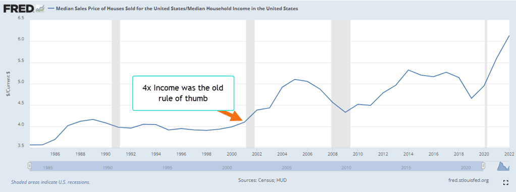
Abel laughed. “There are several characteristics of collective action problems and dealing with the homeless has several of those. People resist multi-family development for fear that it will lower the value of their home. Zoning that permits only single-family housing reduces the opportunities for developers to build more housing. A shortage of housing causes home prices and rents to rise, increasing homelessness.”
Cain interrupted, “Less supply, higher housing costs. Classic supply demand response. But rising home prices are a good thing for an existing homeowner. Naturally, they want policies that preserve the value of their asset.”
Abel nodded. “That’s my point. What’s good for each individual homeowner may not be good for society as a whole. Individual benefit, group loss. Garret Hardin pointed that out in his essay Tragedy of the Commons (Source). Each herder has an incentive to graze their animals on common land, land that no one owns. Together, they overgraze the area and there is no grass for anyone.”
Cain frowned. “Residential land is privately owned.”
Abel argued, “But the zoning is like a common resource. Also, homeowners in single-family zoning are contributing to the homeless problem but paying nothing for the extra city resources needed to deal with the problem. So, they are free riding in a sense, another characteristic of collective action problems.”
Cain finished chewing. Wait. Homeless people are the biggest free riders, but you chose to focus on the hard-working homeowners.”
Abel shook his head. “I’m just pointing out the free-riding aspect of the zoning problem.”
Cain argued, “I hate when liberals say the homeless problem is a zoning problem. Zoning is a relatively small part of the problem.”
Abel replied, “Well, let me finish. Third, there’s the public goods aspect. Presumably, everyone in the city benefits from less homelessness and no one can be excluded from those benefits. Less communicable disease. What else? A sense of pride in the city? And fourth, the homeless detract from people’s enjoyment of public parks, so there’s that aspect of the collective action problem.”
Cain put down his fork. “That’s a nice analysis. Let me come at it from a different angle. Incentives. Look at the incentives to be homeless.”
Abel scoffed, “What? Like free rent?”
Cain argued, “Why do homeless people gather in cities? They like the anonymity. It gives them a sense of independence. They rely on medical services far more than the general population (Source). There are outreach programs available to supply them with food, shelter and clothing. In some cases, inexpensive tents (Source). All of that charity makes homelessness at least more tolerable. One part of the solution is to make it less tolerable.”
Abel interrupted, “What? Put them in jail? Refuse them medical service and let them die? Last week, you said that we should build policies around price incentives. This week, you’re saying let’s build policy on a framework of cruelty?”
Cain smirked. “Give me a break. Last week I said that the price system is thousands of experiments in opportunity costs. Give up this to get that.”
Abel nodded. “The trade-offs act as a counterbalancing mechanism. Homeless people are often beyond the bargaining of trade-offs. In the case of addiction, they’ve already traded their family, their job, their stability for the hamster cage of drug addiction. Those with mental health issues may not be capable of recognizing the choices involved in a trade-off. They may hear voices and imagine conspiracies. Then there are those who are working but are too poor to afford rent in an expensive area. They didn’t voluntarily make a choice to become homeless. Circumstances boxed them in.”
Cain shook his head. “Or there own choices boxed them in.”
Abel argued, “So you’re going to punish them for making bad choices? Isn’t homelessness punishment enough?”
Cain frowned. “Why do homeless people tend to congregate in one area? The police allow it. It attracts more advocates for the homeless who bring food and clothes, the support system that enables their homelessness. The city should prevent such encampments. Why doesn’t it? Policy decisions from liberal politicians who follow Marx’s rule of distributing stuff according to need, not ability. They sacrifice the well-being of their hard-working citizens to tolerate homelessness.”
Abel shook his head. “How many cops want to get involved in restraining and removing people who are not right in the head or on some kind of drug? Cops are likely to quit one police force and join one in a neighboring district where the homeless problem is less acute. It’s a complex problem.”
Cain asked, “So what’s your policy solution?”
Abel shrugged. “Not a solution, but something that would address the zoning aspect of the problem. What if there were a property tax charge for every subdistrict in a city that had single-family zoning? People would then be paying annually for a zoning regulation that they think preserves the value of their property. I would call it an equity insurance fee rather than a tax.”
Cain replied, “I live in a neighborhood that is zoned for single-family homes only. So, I would see a separate charge on my property tax bill for that zoning?”
Abel nodded. “Yes. Connecting the annual cost to the benefit you receive from the zoning.”
Cain raised his eyebrows. “How I would react would depend on the percentage change in my property taxes. If it was another $100 a year, I might not object. But you want to make it cost enough that it would encourage homeowners in a single-family zone to lower their resistance to multi-family development.”
Abel nodded. “That’s the point. I don’t know what percentage increase would do that.”
Cain replied, “Essentially, single-family zoning would become a privilege that only those with higher incomes could afford to pay. Last week, you talked about Make America Fair Again. How fair is that policy to homeowners in older, more established neighborhoods? They are more likely to be retired and on fixed incomes. Already, they resent the increase in their property taxes from higher assessed valuations. Now the city is going to impose yet another fee on them.”
Abel sat back in his seat. “No policy can be fair to everyone.”
Cain objected, “What if there is no visible sign of homelessness in a neighborhood? Homeowners may not see the necessity of such a policy. They will be motivated to vote against it. I like the analysis, though. Shows the complexity of these problems. A viable solution would address all four of those aspects.”
Abel agreed, “You always emphasize the relation between prices and incentives. Homeowners are not incentivized to adopt policies that will increase the supply of housing if it will make the value of their property decline.”
Cain replied, “Exactly. Any policy you put in place will act against that natural tendency. You call it an insurance fee, but since it applies to all homeowners in a district, it acts like a tax. Unlike a price, a tax does not obey the natural forces of supply and demand.”
Abel argued, “A tax raises the price and higher prices reduce demand.”
Cain shook his head. “Yeah, but prices react to something real. They react.”
Abel shrugged. “Can’t see the difference. A tax reacts to something real. In this case, it’s homelessness.”
Cain argued, “The tax you are proposing is an incentive, not a reaction. It is a stimulus you hope will get homeowners to adopt a more lenient attitude toward permissive zoning. Take this, for comparison. A city does not impose a sales tax because they hope it will dissuade people from buying goods. The tax is a reaction to city’s need for revenue to fund the services it provides.”
Abel replied, “So called sin taxes are meant as incentives to get people to buy less.”
Cain laughed. “Don’t try to sell your insurance fee as a sin tax. Owning a home isn’t a sin in anyone’s playbook.”
Abel moved his plate aside. “So, Trump’s tariffs are meant as incentives or punishments and they distort the market.”
Cain nodded. “Before the 16th Amendment, tariffs were the chief source of revenue for the federal government. They served other purposes, yes, but they generated much needed revenue. Today, any tariff revenue would be a drop in the bucket. Trump’s tariffs act as carrots and sticks. That may be the extent of all of Trump’s policies. Carrots and sticks.”
Abel frowned. “There are a lot of carrots and sticks in the income tax code. Tax deductions for college expenses, health insurance, retirement contributions. These are all attempts to get people to do more of something that they would naturally. So how can saving for retirement or going to college distort the market?”
Cain replied, “Tax-advantaged plans were introduced in the 1970s (Source). The financial sector manages trillions of dollars in retirement accounts. That gives it more market share and political power.”
Abel asked, “I take it you’re opposed to any tax whose primary purpose is to influence behavior, not collect revenue?”
Cain drew a deep breath. “I do, but I’m a realist. People get into politics because they want to exert their values, their sense of justice on other people. Now we’ve got someone in the White House who takes that to the limit. I worry for the free market system. I worry for democracy.”
Abel raised an eyebrow. “You weren’t worried last November?”
Cain smirked. “You are more of an institutionalist, but I think I trusted in the institutions that have kept this country together for more than two hundred years. The institutional rules as well as the laws. Seeing long-standing practices fall so quickly has made me question the strength of those institutions. In a political sense, I feel homeless.”
Abel asked, “You think there was insider trading going on while Trump flip-flopped on tariff policy?”
Cain nodded. “Sure. The SEC is not going to investigate. It seems like most of the government is being run by acting commissioners without Senate confirmation. Those of us who complained about the complexity of government are getting a chance to see what it is like when a bunch of loyalists run the government.”
Abel stood up. “I am afraid that we are losing the world’s confidence in American institutions, particularly its currency. I’ll see you next week.”
Cain seemed lost in thought for a minute. “Yeah, next week.”
///////////////
Image by ChatGPT in response to the prompt, “draw an image of a tent with a disheveled person poking his head out of the opening of the tent.”