Interest Rate Ceiling

June 23, 2019

by Steve Stofka

After the Federal Reserve meeting this week, traders are betting on a cut in interest rates in July and the market hit all-time highs. Is a cut in interest rates warranted at this time? Such an action is usually taken in response to weak employment numbers, a decline in retail sales or sluggish GDP growth. Let’s review just how good the economy is.

Unemployment is at 50-year lows. The percent of people unemployed more than fifteen weeks is near the lows of the late 1990s. At almost 18 million vehicles, auto sales are near all-time highs. Real retail sales continue to grow more than 1% annually. In the first quarter of this year, real GDP growth was over 3%. Ongoing tariffs may cause real GDP to decline one percent but a growth rate above 2% is above average for this recovery after the financial crisis.

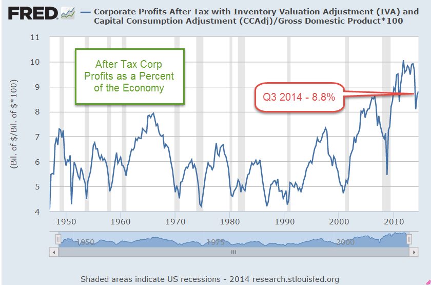
Corporate profits have been strong. In fact, that may account for the volatility of the past two decades. The chart below is after tax corporate profits (CP) as a percent of GDP. The multi-decade norm is in the range of 5-8% but the past twenty years have been above that trend except for the plunge in profits and GDP during the GFC.

Companies have paid part of those extra profits as dividends to shareholders who tend to be cautious pension funds or older, wealthier and more cautious individuals.  Some profits have been used to buy back shares and boost the return to existing shareholders.

Despite the above average profits, investors still have a strong thirst for lower yielding government debt. Why? The Federal Reserve has kept interest rates below a market equilibrium, which is currently about 3.8%, far above the current 2.4% federal funds rate (Note #1). As with any price ceiling, the below-market price creates a shortage. In this case, the shortage is in the capital investors want to supply to governments to meet the demand for capital. Consequently, investors have been searching for alternative substitutes or near-substitutes. That distortion is being reflected in stock market prices.

Despite a strong economy and corporate profits, the SP500 has gained less than 5% from its peak high in February 2018 after the passage of the 2017 tax cuts. Including dividends, the SP500 has gained just 5.7% in 16 months. If we turn the clock back a few weeks to the end of May, the total return of the SP500 during the past fifteen months was a big, flat zero. Those gains of the past sixteen months have come in the past three weeks on the hope and the hint of rate cuts.

An intermediate bond ETF like Vanguard’s BIV has returned 5.2% in the same period. On a scale of increasing risk 1-5, with 1 being a safe investment, BIV is rated a 2. The SP500 is rated a 4. Investors buying the broad stock market have not been rewarded for the additional risk they are taking.  How long will this situation persist? For as long as the Fed keeps a price ceiling on interest rates.

///////////////////

Notes: A popular model of equilibrium interest rates is the Taylor rule proposed in 1993 by John B. Taylor, a member of the Council of Economic Advisors under three presidents. The Atlanta Fed has a utility that calculates the current rate and allows the reader to change the parameters. Click on the graph icon, accept the default parameters and the utility graphs the equilibrium rate and the historical Fed funds rate.

Economic Cracks

February 17, 2019

by Steve Stofka

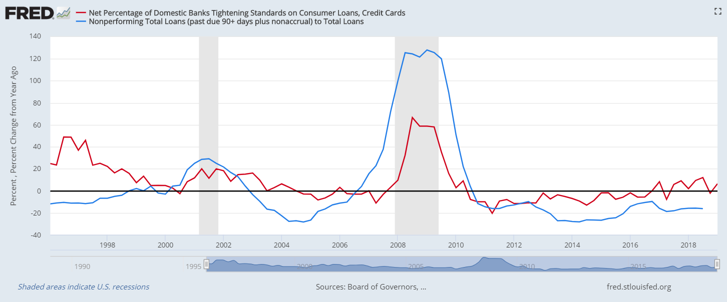
As the recovery enters its tenth year, there are signs of strain. As debtors struggle to pay their loans in a weakening economy, the percentage of non-performing loans increases.  The current rate of one percent indicates a healthy economy (Note #1). When the annual change in the rate of delinquency increases, that has been a reliable indicator that the economy is growing stagnant. Here’s a chart of the percent change in non-performing loans. A change above zero has preceded the last three recessions.

Non-PerfLoansChange

Let’s add one more series to the graph to help us understand the cycle of consumer credit. In the graph below, the red series is the percentage of banks tightening lending standards. Notice how the banks respond to a rise in delinquencies by being more selective in their credit criteria. Eventually, this tightening of credit leads to a recession. The cycle is as natural as the ocean currents that distribute heat around the planet.

NonPerfBankTighten

The financial news agency Bloomberg reports that delinquent auto loans are the highest since 2012 (Note #2). Bankrate reports that credit card debt has risen since last year. Less than half of people surveyed have emergency funds (Note #3).

December’s retail sales report, released only this week because of the government shutdown, showed a surprising decline of 1% from November. Have some consumers reached their limit? Retail sales, adjusted for inflation and population growth, does not show the strain so far. Look at the period from late 2015 through late 2016 when sales growth consistently slowed below 1%. That was a key factor that cost Hillary Clinton the election. Trump turned voter dissatisfaction into an electoral victory in the Midwest.

RetailRealAdjPop

Politicians ride to power on the anger of voters. In 1994, Republicans overcame forty years of Democratic rule in the House by promising less regulation and lower taxes in a “Contract with America.” When the Supreme Court decided the 2000 election in favor of a Republican president, they enacted tax cuts to reverse the tax increases passed by Democrats in 1993. In 2006, voters were angry with the incompetent Bush administration and reinstalled Democrats in the House.

In the depths of the Financial Crisis in 2008, Democrats rode a wave of anger, despair and hope to take the White House and command a filibuster proof majority in the Senate for the first time since the post-Watergate Congress thirty years earlier. Such a rare majority indicated that voters strongly wanted a solution to the crisis (Note #3). The Obama administration and Democratic Congress protected the financial and insurance industries while ordinary people lost their homes and their savings. The one piece of legislation that emerged from that majority was Obamacare, the bastard child of back alley compromises between mainstream Democrats and the health care industry. Few who voted for it knew what was in the bill.

In 2010, Republicans rode the anger wave of the Tea Party caucus to retake the House. With an equal number of Senate seats up for re-election, Republicans took six seats from Democrats and ended their filibuster proof majority (Note #4). In 2014, voters handed the Senate back to Republicans, then gave the reins entirely to the Republicans with the election of Donald Trump to the presidency in 2016.

In 2018, Democrats rode a wave of anger to take back control of the House. Social media campaigns whip up indignation to fan the flames of voter anger in the hopes that Democrats can at least take back the presidency in 2020. Voters may not be in enough economic distress to give Democrats control of the Senate in 2020, but it is the Republicans who have the most seats up for re-election this coming Senate cycle (Note #4).

Credit expands and contracts in a seasonal multi-year cycle. Banks are tightening in response to higher delinquencies. Will the timing of the credit cycle coincide with the 2020 election?

///////////////////////////

Notes:
1. In 2016, China, Japan and Germany had rates below 2%; the U.K. and Canada had less than 1%. On the high side, Greece had 36%; Italy had 17%, and Spain had 7%.
2. Why are so many people delinquent on auto loans? Bloomberg
3. In 1964, the Supreme Court forced the states to redistrict their state legislatures based on population changes. For fifty years, Democrats were sometimes able to forge filibuster proof Senate majorities because racist Southern states were effectively one party Democratic states. Reynolds v. Sims . Since the ratification of the 17th Amendment in 1914, Republicans have never had a filibuster proof majority
4. A third of Senators are up for election every two years so party advantage shifts with every election cycle.

Consumer Credit

It is very iniquitous to make me pay my debts; you have no idea of the pain it gives one. – Lord Byron

October 7, 2018

by Steve Stofka

The total of all consumer loans, excluding mortgages, is almost $4 trillion. The Federal government owns $1.5 trillion of that total, most of which is student loans, which have tripled in the past decade. According to the Dept. of Education, 11% of student loans are in default, three times the credit card default rate and more than ten times the auto loan default rate (Note #1).

Over a five-decade period, the stock market has risen when consumer credit rose. Below is a chart of consumer debt outstanding as a percent of GDP (Note #2).

ConsCreditPctGDP

This a decade long indicator, not a timing tool. Notice that the ratio of credit to GDP (blue line) rises during recessions (shaded gray) when GDP, the bottom number in the fraction, falls. When the recession is over, credit falls as people fall behind in their payments, loans are written off, etc. Now GDP starts rising again while the top number, credit, is falling.

Auto loans make up 28% of outstanding consumer credit and currently have less than a 1% default rate. If we adjust the total of consumer credit by the extraordinary growth in student loans, auto loans make up 39% of total consumer credit (Note #3). We saw a similar percentage in the mid to late 1980s when savings and loans aggressively extended auto loans and mortgages. In the late 1980s and early 1990s, a third of all S&Ls failed.

Typically, people do not count vehicle depreciation in their budget, but they should, just as businesses do. Example: the average yearly take-home pay is $52K. Let’s say the average car, new and used, is $24K and depreciates $2400 a year (Note #4). Let’s say that the average person saves about $2400 a year to make the math easy. The $2400 that goes in the savings bank is simply offsetting the $2400 in depreciation. There is no savings.

In addition to depreciation, many of us don’t include the cost of inflation in our budget. Six years from now, a replacement car, new or old, could cost an additional 15%. Without adjusting for these “hidden” costs, we may think we are getting by. Over time, however, we add these hidden costs to our credit balances. We put less down on the next car and get longer auto loans. The average loan length is now 5-1/2 years. As soon as we are done paying off one car, it is time to get another (Note #5).

The economy is strong, and it needs to stay strong so that households can pay back their loans. The ultra-low interest rates of the past decade have reduced the monthly debt payments for many. For the past two years they have leveled at 5.6% of disposable personal income, the mid-point of the past forty years. For every $20 that a person takes home, they are paying $1 to service their consumer debt. The average yearly debt service payment would be about $3000 on a $52K take-home pay.

In response to the strong economy, the Federal Reserve has been raising interest rates to a more normal range. The 30-year mortgage rate just hit 5% this past week. Rising interest rates raise the monthly payments and reduce the loan amounts that borrowers can qualify for.  Many younger workers are unfamiliar with a world of normal interest rates.  They will have to learn a new math.

////////////////////////////

Notes:

1. Student default rates . Default rates reported by the credit agency Experian .
2. More detail on consumer credit here at the Federal Reserve ()
3. I made the adjustment by subtracting $1 trillion in Federal student loans from the current total of credit. This pretends that Federal loans grew 15% in the past decade, not 300%.
4. The average amount financed on a used car is $17,500 (FRED series DTCTLVEUANQ). New car loans average $29,800 (FRED series DTCTLVENANM).
5. A buyer of a new car holds it for 71 months according to Auto Trader.

////////////////////////////

Misc

Amy Finkelstein is a MacArthur genius award recipient who studies trends in health care. Proponents of Medicaid expansion projected that lower income families would better control and plan their medical care under Medicaid. Instead they have used the ER even more.  She found that people visit the ER more, not less. Although families report better health and more confidence in their financial security because of Medicaid expansion, measureable health outcomes have shown no change. WSJ article (paywall) is here. Her citations on Google Scholar.


Package Me

July 9, 2017

Two weeks ago I looked at a long term trend of consolidation and concentration. Technology companies now dominate the top spots in the SP500, the number of retail outlets is shrinking, the number of banks is dwindling, and the population itself is concentrating in urban areas. This week, I’ll look at a companion trend – categorization.

The essential business model of some leading technology companies is the selling of advertising to us and the selling of us – our interests and choices – to other companies. We are the consumers and the products. We are the components of the business models of companies like Facebook (FB) and Google.

A business model is a plan to provide and capture value. FB and Google provide value by connecting us to each other and to a vast trove of information, most of which we ourselves provide. FB and Google capture value by selling us. To sell us, the unique composite of all of our choices must be packaged into algorithmic categories.

We consume information and we are information. We are part of the network of information. When I travel, Google Maps tells me where I am and how to get where I want to go. Where is a grocery or sporting goods store along the way? Google knows. Within hours, Google has sold that information to companies who offer me deals on hotels and restaurants. I am part of the network.

Listen to a forty year old song from Pink Floyd, Welcome to the Machine. It is a cynical vision of being absorbed into the dream machine of the entertainment industry. This is a brave new world of information – and maybe some disinformation and some anger and scams and sexploitation but I want to focus on the positive.

As I drive to work or the store, I give a wave to the mobile purchasing unit in the car next to me. Hi, neighbor! I don’t mind that my entertainment, dining and transportation choices are for sale. I do mind that my political and religious beliefs are packaged and sold like commodities. That is the price that I pay for being in the information club.

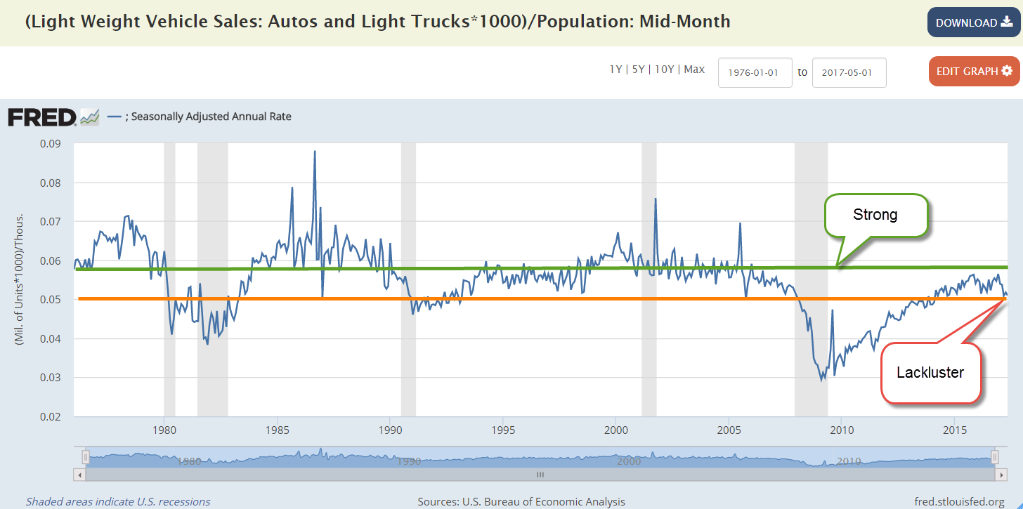
Talking about travel….annualized sales of autos and light trucks has fallen below 17 million for several months now. On a per capita basis, sales never reached the levels of past economic recoveries. We are buying about 5 cars for each 100 people, and that is less than the 5.8 cars we have bought in previous periods of economic strength. The auto industry would have to sell almost 19 million cars and light trucks each year to meet those per capita levels.

AutoSalesPerPop

I heard someone remark that cars are becoming like appliances. As I drive down the highway, I see that there are only a few body styles. Engineers have gradually perfected those designs that minimize wind resistance in order to increase gas mileage enough to meet EPA requirements. I drove next to a Ford Fairlane 500, a boat of a car from the era when car designers and advertising guys – always guys – teamed up and let their creative juices flow. Those were the days when a car was a signature. Now I drive down the highway in a category of vehicle. Hey, ma, look at me!

In order to sell me stuff, Google and FB need my attention. Unfortunately, I must devote a lot of my attention to driving. As a mobile purchasing unit, this is an unproductive use of my attention. A self-driving car will be the final step in the appliancification of the automobile. “Google, when will I arrive at work?” “In approximately 8 minutes.” Beam me up, Scotty.

Over a million people in the U.S. die in automobile accidents each year, and approximately 10% of the entire population are injured in a year. The major car companies have committed to having a driverless car by 2020 or soon after. The cost to add driverless capabilities is only a few thousand dollars. Some research companies are predicting (Motley Fool article) a gradual transition to driverless cars with 10% being fully autonomous in 15 years.

I think that the changeover will happen more quickly because Google and FB need my attention. Thousands of vendors want the dollars in my pocket to join the network. For the next 10 minutes only I can get a deal on a fresh pastry and a coffee at the Starbucks just down the street. Say or press “Yes” to accept this deal and my car will drive itself into the Starbucks’ drive-up lane.  Would I like to order ahead?  The car can do that for me. Well, sure.  Hey, I like this new world.

I wrote about consolidation and concentration a few weeks ago. Soon to come will be an integration to package us as mobile purchasing units. A big technology company could partner with or absorb a finance company to help me buy a driverless car in order to market to me. Google could subsidize a better interest rate on my auto loan or lease as a cost of packaging my choices to other vendors. I hear the sound of dollar bills stirring in my pocket. They want to be part of the network as well.

Next week, the stream and the pool…

Sales Tax Collections

January 8, 2017

The New Year begins, the 9th year of this blog that began during the financial crisis.  For two decades I had studied financial markets but the financial crisis surprised most people.  This was my attempt to organize and share my thoughts.

Sales Tax Collections

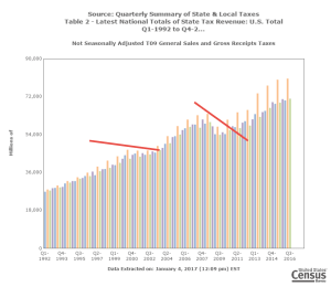
Let’s look at a data point that has been a consistent indicator of economic health – sales tax collections. This is not survey data or economic estimates but actual tax collections based on consumer purchases. For the first 3 quarters of 2016, sales tax collections are up 1.6% above the same period in 2015. (Census Bureau)    As we will see, this tepid growth rate does not compare well with the historical data of the past 25 years.  Below is a quarterly graph of sales tax collected in the 50 states.

As we can see in the graph above, the 2nd quarter (orange bar) is the highest each year, and is a good indicator of consumer activity and confidence. Since population growth is about 1%, the annual growth of sales tax collected should be above that mark to be effectively positive.

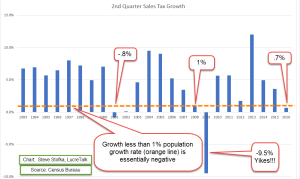
In the graph below, we can see negligible or negative growth in 2001, 2008 and 2016. In 2001 and 2008, we were already in recession, although it took the recession marking committee at the NBER almost a year to declare the beginning of those recessions.  By selecting the 2nd quarter growth rate in the historical data, we can more easily see the weakness at the start of an economic downturn.

In retrospect, 25 years of data is rather sparse.  We can only hope that this year’s lack of sales tax growth may turn out to be a warning sign only, a fluke.  Third quarter tax collections were effectively positive, but only 2% growth, and that annual growth has consistently declined in the past three years in a pattern exactly like the weakening of 2006 – 2008.

Of particular note in the graph above is the steep 10% drop in sales tax collections in the second quarter of 2009. Fom a vantage point eight years in the future, we may have forgotten the degree of fear during the winter of 2008-2009.  The American people were holding onto their money.  State budgets were crippled by the lack of sales tax collections, an important and ongoing source of revenue for state and local governments.

See end for a side note.

////////////////////////

Population Growth

Business Insider published a chart of 2015-2016 population data from the Census Bureau.  We can see a clear shift from the northern states to the mountain and southern states.  Retiring boomers, who want to maximize their fixed incomes, will shift from states with high state income and property taxes like New Jersey and New York, and move to states with lower taxes.

///////////////////////

Tax Reform

In a few weeks Republicans will control the legislative machinery, and have promised  tax reform that, after thirty years, is overdue.  One of the proposals on the bargaining table is the end of the home interest deduction, which prompted this blog post at Slate.  The author contends that the elimination of this deduction will hurt middle class homeowners, who will see the value of their homes decline by 7%.

I’ll add in some contextual data from the IRS.  In 2011, 22% of the 145 million (M) returns claimed mortgage interest totalling $321 billion. ( IRS tax stats Table 3) People making a middle class income of less than $100K claimed half of that interest – 14% of all returns.  The average interest deduction for these middle class households was $8100.

Two million returns with incomes of $500K and above claimed $46B in mortgage interest, about 15% of the total interest claimed.  For these high earners, the average deduction was $20,000.

The tax reform of 1986 eliminated the interest deduction on credit cards and cars, but lawmakers could not go the final distance and squelch the home mortgage interest deduction.  At the time, auto dealerships complained that, without the interest deduction on new car loans, their business would suffer.  Tax subsidies affect both consumers and the businesses who are indirect recipients of the subsidy. Should 78% of taxpayers subsidize the housing costs for 22% of taxpayers?   Certainly, the 22% appreciate the subsidy! The real estate industry continues to resist any tax changes that might have a negative impact on their business.  Each industry deserves a subsidy of some kind because that industry is important to the overall economy – or so the argument goes.

///////////////////////

The End of Capitalism – Almost

Let’s get in the wayback machine and dial in 1997.  The dot-com boom is not yet a bubble but is growing.  Cell phones are growing in acceptance but the majority of people do not have one.  A one year CD is paying more than 5%.  The unemployment rate is about the same level as today (2016).  What is very different between then and now is the number of publicly traded companies.  In 1997, there were over 9000 listed companies.  Today, there are about 6000 companies.  The 2002 Sarbanes-Oxley (SB) law has such stringent and plentiful financial reporting regulations that many companies decide not to go public, or to sell themselves to a larger company that already has the internal infrastructure in place to comply with SB regulations.  Both parties want to repeal or amend the law but cannot agree on the details.  Readers can click for more info.

//////////////////////////

Next week I will compare the 10 year performance and risks of various portfolios.  There are some surprises there.

//////////////////////////

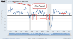
Side note on Sales Tax.  The Federal Reserve charts retail sales but these are based on data samples and will not be as accurate as the actual tax collected.  When retail sales are adjusted for inflation, the year over year growth can give a number of false positives.  In the graph below, I have marked up periods that went negative without the economy going into recession.  I think that the actual tax collected may be a much more accurate predictor of economic weakness.

New Year Review

January 3, 2016

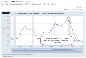
As we begin 2016, let’s take a look at some trends.  It is often repeated that the recovery has been rather muted.  As former Presidential contender Herman Cain once said, “Blame Yourself!”  You and I are the problem.  We are not charging enough stuff or we are making too much money. Debt payments as a percent of after tax income are at an all time low.

At its 2007 peak, households spent 13% of their after tax income to service their debt.  Currently, it is about 10%. In early 2012, this ratio crossed below the recession levels of the early 1990s.  By the end of 2012, this debt service payment ratio had fallen even below the levels of the early 1980s.  Almost six years after the official end of the Great Recession the American people are behaving as though we are still in a recession.  An aging population is understandably more cautious with debt.  In addition to that demographic shift, middle aged and younger consumers are cautious after the financial crisis. We gorged on debt in the 1990s and 2000s and paid the price with two prolonged downturns.  Having learned our lessons, our overactive caution is now probably dragging down the economy.

In this election year, we can anticipate hearing that the sluggish economy can be blamed on: A) the Democratic President, or B) the Republican Congress.  It is Big Government’s fault.  It is the fault of greedy Big Companies.  Someone is to blame.  Pin the tail on the donkey.  Blah, blah, blah till we are sick of it.

************************

Auto Sales

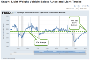
The latest figures on auto sales show that we are near record levels of more than 18 million cars and light trucks sold, surpassed only by the auto sales of February 2000, just before the dot com boom fizzled out.  On a per capita basis, however, car sales are barely above average.  The thirty year average is .054 of a vehicle sold per person.  The current sales level is .056 of a car per person.  Automobile dealers would have to sell an addiitonal 900,000 cars and light trucks per year to have a historically strong sales year.

************************

Construction Spending

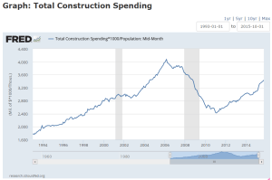
In some cities, housing prices and rents are rising, and vacancies are low.  We might assume that construction is booming throughout the country.  Six years into the recovery per capital construction spending is at 2004 levels and that does not account for inflation.  Levels like this are OK, not good, and certainly not booming.

*************************

Employment

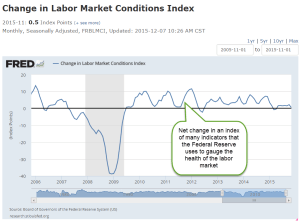
The unemployment rate and average hourly wage may get most of the public’s attention but the Federal Reserve compiles an index of many indicators to judge the health of the labor market.  Positive changes in this index indicate an improving employment picture.  Negative changes may be temporary but can prompt the Fed to take what action it can to support the labor market.  Recent readings are mildly positive but certainly not strong.

*************************

Stock Market

Many of the companies in the SP500 generate half of their revenue overseas.  Because of the continuing strength of the dollar, the profits from those foreign sales are reduced when exchanged for dollars.  According to Fact Set, earnings for the SP500 are projected to be about $127 per share, the same level as mid-2014.  In the third quarter of 2015, the majority of companies reported revenue below estimates.  As 4th quarter revenue and earnings are released in the coming weeks, investors will be especially vigilant for any downturns in sales as well as revisions to sales estimates for the coming year.  It could get bloody.

Glootch or Glut?

March 15, 2015

Retail

Indicators of business activity and confidence have all been strong.  The Purchasing Managers Index, the monthly employment report, and the NFIB small business index have shown exceptional strength in the past several months.  A week after a strong employment report came the worrisome news that retail sales declined for the third month.

A 2% drop in auto sales was the primary driver of February’s decline but the lack of demand is evident in the broader economy.  Excluding auto sales this is the second three month period of declining sales since the recovery began.  Following the slump in 2012, the SP500 sagged about 7%.  The market’s response to this slump has been muted so far.

American businesses had hoped that their customers would spend the dollars saved at the gas pump but consumers may be tucking away some of that cash. The slowdown in retail sales may be partly due to the harsh winter in the east, or a lack of income growth.  The strong dollar has made American products more expensive to export so businesses are especially dependent on domestic demand. Since last summer, prices at the wholesale level have declined steadily.  Commodities other than oil are also showing slack demand.

The inventory to sales ratio has climbed abruptly in the last half of the year.  Businesses make their best guess in anticipating future demand.  A capitalist economy is based on the decision making of millions, not a central committee of a few.  If inventories continue to mount, we can expect that businesses will adjust to the new environment and rein in production and expansion plans.

*************************
Retirement

Twenty years ago I read articles on portfolio diversification like this one and was glad that I wasn’t old enough to be concerned about that kind of stuff.  Then one morning I was shaving and noticed that I was developing a slight turkey wattle in my neck, the same thing I had noticed in my Dad. OMG! I was getting old!
A Bankrate.com blog post features a chart of savings goals that a person at each stage of life should have accumulated to ensure that they can maintain their living standard in retirement.  The benchmarks are based on one’s current income.  Many Americans do not even meet these modest goals.  According to the chart, a person making $60K  who retires at 67 should have $500K in savings and investments.  
*************************
Apple
Telephone and radio were the high tech firms of the early 20th century.  In 1916, ATT was added to the Dow Jones Industrial Average (DJIA), acknowledging that the company had become a pillar of the American economy. 
At the close of trading on March 18th, almost a hundred years later, ATT will be dropped from the DJIA and replaced by Apple, a high tech firm of the 21st century.  Apple’s projected earnings growth for this year may cancel out the anticipated negative earnings growth of the DJIA but Apple is a more volatile stock than stodgy ATT so daily price changes in the index are likely to be a bit more dramatic.
*************************
Budgeting
Last week, economist Greg Mankiw wrote a piece in the New York Times explaining the recent change from static to dynamic budget scoring in the new Congress.  These are two different methods for estimating the effects of proposed tax changes on the budget over the following ten years.  Static scoring, the previous system, has been in place for decades and assumes no changes to the economy resulting from the proposed tax changes.  Dynamic scoring estimates changes in GDP and revenues resulting from the tax changes. Several examples illustrate differences between the two types of scoring.  The article is well written and easy to understand without the use of complicated economic models.

Gangbusters!

December 7, 2014

On Monday, George intended to put the $50K from the CD into the bond market. He couldn’t decide between a long term bond index like Vanguard’s BLV or TLT, the ETF that tracked 10 year Treasury bonds. Both the bond and stock markets opened lower in the morning which confused him and he did nothing. Gallup released their monthly survey of consumer spending for November, showing a respectable gain of more than 4% over last November.

Tuesday’s report of auto sales in November was strong.  Total vehicle sales topped 17 million on an annualized basis. Auto manufacturers reported particularly strong sales over the Thanksgiving holiday.  SUVs were big sellers and that was a double plus for auto companies because those vehicles had larger profit margins.  The American car buyer has long had a short memory.  Six months of falling gas prices prompted many to abandon their economical cars and wrap themselves in a big bubba vehicle.

Construction spending was up 1.1% from the previous month and 3.3% above last October.  The economies of Europe may have slipped into neutral or recession but the U.S. economy was chugging along.  The upbeat reports gave the stock market a minor boost but there was little selling of Treasuries, indicating a growing split in sentiment among investors.  George decided to put his and Mabel’s CD money into TLT.

On Wednesday, the Centers for Medicare and Medicaid Services released their annual report on health care costs.  Spending had increased only 3.6% in 2013, the lowest increase since 1960, and the fifth year in a row that spending had grown less than 4%.  Out of pocket expenses had risen from $293 billion in 2007 to $339 billion in 2013, a 16% increase over six years.  Before the recession, George could remember years when spending rose almost that much in a single year.  CMS reported that consumers’ out-of-pocket spending was only 3.2% of charges, less than the 5.9% of charges in 2007.

CMS published a historical table that caused George to raise both eyebrows.  In 1960, Americans spent $125 ($967 in 2012 dollars) per person on health care. In 2012, that figure had grown eight-fold to $7533 per person.  Administrative and public health programs added another 15% to those costs.  In 2013, the total cost per person was over $9500 for a whopping national total of $2.9 trillion spent on health care, almost 18% of GDP.

While families were shelling out more for health care, companies were grabbing a larger share of the economic pie.  As a percent of GDP corporate profits had been trending upward since 1990.

The private payroll processor ADP reported private job gains of 208,000, slightly below expectations but still above the 200,000 mark considered a healthy job market. Later that day came the announcement that a Staten Island grand jury decided that there would be no indictment in the death of Eric Garner.  Caught on video, five or six officers had surrounded the man to arrest him for selling bootleg loose cigarettes.  One of the officers put a choke hold on the unarmed Garner, restricting his breathing till he died of asphyxiation.

Later that day, four Denver bicycle cops were escorting a parade of students protesting the grand jury decision in Ferguson.  Acting as a buffer between the students and traffic on the busy street east of the Capitol, the officers were struck by a Mercedes as it ran through an intersection.  The Mercedes dragged one of the officers about thirty yards and that officer was taken to the hospital in critical condition.  On the evening news, George and Mabel learned that the driver of the Mercedes might have been having a seizure when he hit the officers.

Late Thursday morning, George was focused on several economic reports.  Since 2010, the polling firm Gallup had conducted a simple employment survey, called P2P, that counted the number of people who had worked for money in the past week or had looked for work in the past week.  Gallup reported the lowest unemployment rate, 6.2%, since the poll began.  New jobless claims were one again just under 300,000, indicating that the previous week’s 314,000 might have been an anomaly.  The 4 week average of new claims was still below 300,000.

Friday morning the reporters dusted off their sports dictionaries as they searched for words to describe the monthly labor report from the BLS.  Blockbuster.  Gangbusters. Blowout numbers. Spectacular.  Amazing.  George poured another cup of coffee. Yes, 321,000 new jobs sounded great!!! Too great. George got out his magnifying glass, put on his Sherlock cap and went hunting.  First of all, ADP had reported 208,000 private job gains.  The BLS report included new government jobs which the ADP did not include.  So back out the 7000 new government jobs to get private job gains of 314,000 according to the BLS.  Paging Dr. George, number surgeon.  He took out his skeptical scalpel. Take the average of the two estimates, which was 314 +  208 = 522, divided by 2 = 261.  Add back in the 7000 government jobs and probably the more accurate figure was close to 270,000 – 280,000.  September’s job gains had been revised up 20,000 by both ADP and the BLS. The BLS also revised the job gains of October,  getting closer to the averaging method that George used. Sacre bleu!  Averaging really works!  George was a big believer in averages.

Anyway, the employment report was strong, just not as fantastic as it first appeared. Average monthly job gains for the past year had been about 230 – 240,000.  George picked up his magnifying glass.  Hmmm, he said.  Retail job gains were 50,000, far above the 22,000 average of the past year.  At least 20,000 of those job gains were temporary seasonal gains.  Let’s be generous and start with 280,000 jobs. 280 – 20 = 260.  Now job gains were approaching the average of the past year.

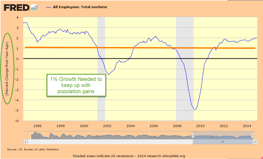
Still, the yearly growth in employment was climbing toward 2%, slowly but surely getting stronger.

Professional and business service jobs had been a leading sector for the past few years and were especially strong this month at 86,000, way above the average gains of 50 – 55,000.  George raised a skeptical eyebrow.  A closer look showed that the strong gains were particularly strong in bookkeeping and accounting.  Take out 20,000 temporary tax jobs, George thought, and now his count was down to 240,000.  Boy, this was quickly becoming an average employment report.

Yearly gains in hourly earnings for the average worker were just under 2.2%, just barely ahead of inflation. For all workers, the gains were 2.1%.

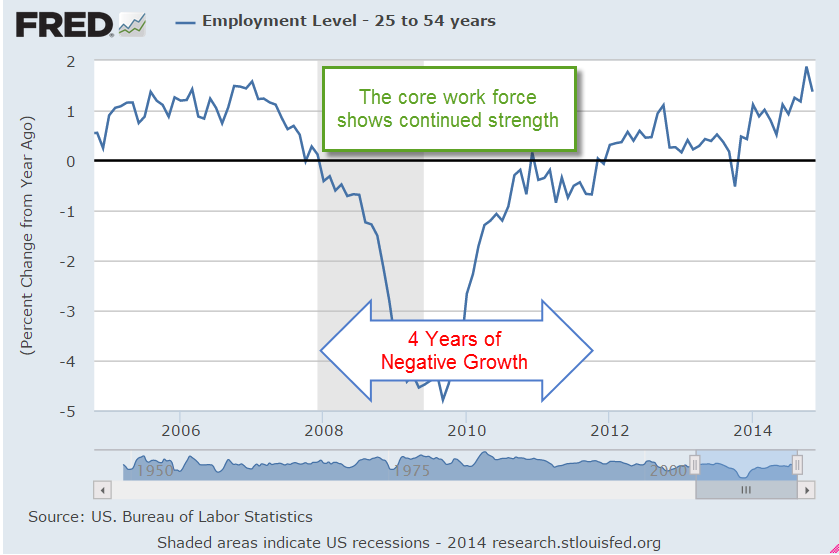
George put away his magnifying glass and put on his rosy glasses.  The average hourly work week had increased .1 hour over the past month, a good sign.  However, that was also the yearly gain.  Not so good.  George cleaned his rosy glasses.  The gains had been fairly broad and the core work force aged 25 – 54 had increased to nearly 96 million.

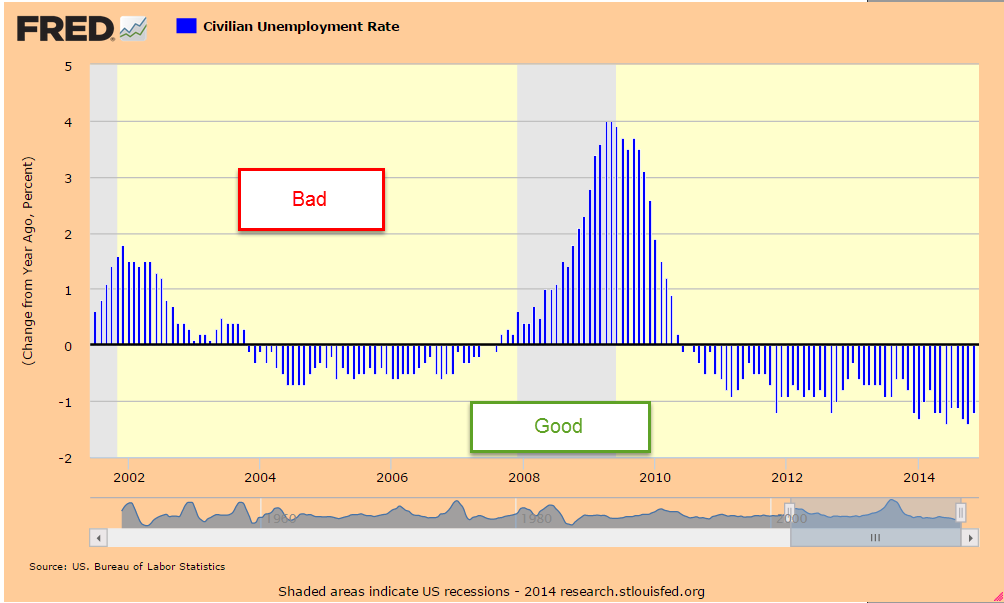
The construction and manufacturing sectors reported strong gains.  Although the headline unemployment rate remained the same at 5.8%, this rate was more than 1% below last year’s rate, a sign of a relatively healthy labor market.

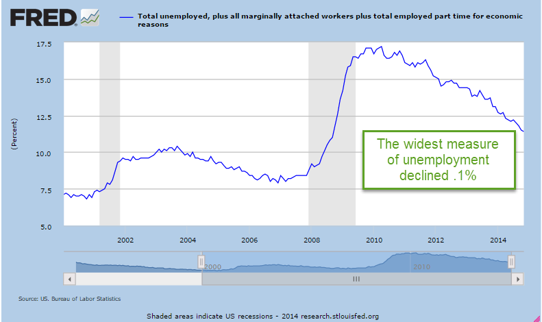
A wider measure of unemployment, the U-6 rate, had declined .1% but was still above the rates in the mid-2000s.  George needed a better pair of rosy glasses.

George checked to see if the Federal Reserve had updated their Labor Market Conditions Index but that would probably come next week.  The market had risen a few tenths of a percent since the high of two weeks ago.  According to a Fact Set report, earnings growth for the fourth quarter had been revised down from 8.3% to only 3.4%.  After rising up almost 14% since the mid-October trough, the SP500 had stalled despite a number of positive reports.  Treasury bonds had lost a few percent in price since mid-October but had stayed relatively strong, indicating some skepticism toward any further stock gains.  The stock market seemed to be treading water ahead of the December 11th deadline for Congress to pass a spending bill.  Despite promises that there would be no government shutdown this time, investors might be a bit less confident in the dependability of promises from the Republican leadership.

Adjusting the Carburetor

November 9, 2014

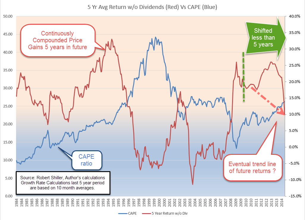
About two thirds of companies in the SP500 had reported earnings for the third quarter. George guessed that positive earnings surprises were somewhat above the normal 70% but as former Presidential contender Herman Cain said, “I don’t have facts to back that up.”  Checking his guess, George went to Fact Set which provides a weekly update summary of earnings reports.  Positive earnings surprises were the highest percentage in over four years. On the other hand, Fact Set was reporting that the forward price earnings ratio of the SP500 was above the 5 and 10 year average.  Einstein famously quipped that the most powerful force in the universe was compound interest.  He might have mentioned an equally powerful force – reversion to the mean.

George updated his spreadsheet with data from Robert Shiller, the Yale economist who had devised the CAPE ratio, an inflation adjusted Price Earnings ratio for the SP500.  When the CAPE was higher than average, as it had been the past two years, price gains over the following five years were likely to be low or negative.  George had added a spreadsheet column to measure the annual percent gain in stock prices five years in the future, then plotted these five year gains against the CAPE ratio.  In the long run of several years, the above average gains in stock prices of the past few years were likely to drift lower or turn negative, bringing their 5 year return to the post-WW2 historical mean of 7%.

But in the post-WW2 period, the stock market had almost always gained in the year after a mid-term election.   It’s like a junction on a hiking trail with many signs and no mileage, George thought.

Monday’s report on auto and truck sales was almost exactly in the middle of the range of expectations.  Promotional sales in August before the introduction of 2015 models had propelled sales upwards in August. Sales in September and October had stayed on trend, a sales curve that was flattening.

Manufacturing data from ISM was strong and continuing to rise, but the market seemed to be in pause mode a day before the elections.  “One more day!” Mabel exclaimed. “We’re being bombarded with political ads.” George reflected on that for a second. “I don’t think I’ve actually seen one ad,” he said.  “We buzz through them when we’re watching a program.”  “Well, sometimes I like to watch the local news live or the weather channel,” Mabel responded.  “It’s become impossible to watch anything live on TV.”  George wondered how many millions would be spent on this election.  How many voters were like he and Mabel, paying little if any attention?  Mabel was a straight ticket voter.  It took her less than ten minutes to vote.  Amendments to the Colorado Constitution – no. “Don’t you even read them?” George had once asked her.  “Nope, they’re all sponsored by special interests,” she had replied.  “What about the marijuana amendment two years ago?” George had asked. “Well, I did vote yes on that one,” Mabel had conceded.  George spent hours researching candidate bios and their positions on the issues.  He would sometimes bring up a name of an independent candidate or a Libertarian candidate to Mabel.  “Why waste your time?” Mabel had asked.  “Whether we like it or not, we’ve got a two party system in this country.  Pick one and vote.  No Independent or Libertarian candidate is going to win.” “Yeh, what about Ross Perot in ’92?” George had asked.  “Cost Bush the election,” Mabel had responded. “No, it didn’t.  Perot took about as many votes from Clinton as he did from Bush,” George had argued.  Where had he read that?  Probably Wikipedia.  “Fine,” Mabel had countered with that tone of voice meaning end of argument.

As they watched election results on Tuesday, George commented that he had been wrong.  “No!” Mabel exclaimed, her hands raised in supplication to the fates.  “Let me write this down,” she said. “Hecklers, always the hecklers,” George shook his head in a mock display of discouragement. “No, really.  I thought the Republicans would gain the Senate but just barely.  Gardner is cleaning Udall’s clock.  Look at Mia Love in Utah.  Methinks there’s a change in the wind, oh forsooth.”

Colorado was a toss-up.  As they turned in for the night, one channel had declared the Republican gubernatorial candidate, Bob Beauprez, as the winner in the race.  In the state senate and house, the Democrats held a slim majority that could be overturned but the races were too close to call.  George expected a bump up in the market the next day unless ADP, the private payroll processor, had a disappointing report of private job gains.

Wednesday morning they woke to the news that incumbent Colorado governor John Hickenlooper had squeaked out a win but his rival had still not conceded.  State senate and house races were still undecided and there might be recounts through November. “If this were a baseball or football game, this would be exciting.” George’s banter had little effect with Mabel who was in a rather sour mood. “Look,” he added, the Dems will have a chance to take back the Senate in 2016.  The Republicans will have six or seven Senate seats up for grabs by the Democrats.  It’s the math of Senate elections.”

In addition to gaining the Senate, Republicans had extended their control of the House.  George turned to the ADP report of private job gains – 230,000.  The market had popped up about 1/2% at the open, showing a curious restraint after the previous night’s Republican sweep.  One of their CDs would be due in a few weeks but George knew this was not a good time to bring up the subject of moving some of that really safe money into something else.  Their son Robbie, his wife Gail and their grandson Charlie would be coming over this weekend and that would help brighten up the mood in the house.

The price of West Texas Intermediate crude oil crossed below the $80 mark.  The game was on to control the world market for oil.  Fracking in the U.S. had increased supply, reducing net imports of oil by the U.S.  However, the cost per barrel using fracking methods is more expensive than conventional drilling.  The only way that the Saudis could strengthen their dominance of the market was to drive the price down to a point where fracking was no longer profitable, putting pressure on these suppliers.  At a price below $80, plans to start new wells might be put on hold.  At a sustained price below $80, some suppliers with higher drilling costs might shut down or reduce their output.  Russia, Venezuela and Mexico depended on a higher oil price to fund their governments and social programs.  The lower revenues from oil were exerting a lot of political pressure within these countries.

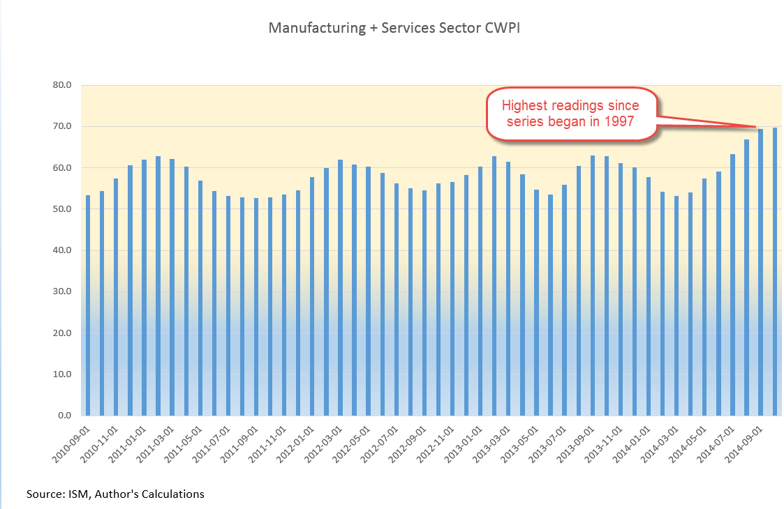
ISM released their monthly report on the service sectors.  George added the new data to his spreadsheet. He had expected a decline from September’s peak, but the composite of manufacturing and non-manufacturing was as strong as September.

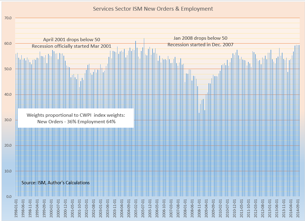
Employment and New Orders were two key factors in the services sector.  For the fourth month in a row, the readings pushed the 60 level, the boundary between strong growth and robust growth.  There had only been two times in 2005 when readings had been this strong.

 On Friday, the BLS released their monthly report of employment gains.  Although net job gains were slightly below expectations, there were gains in most industries, a healthy sign.  As usual, George averaged the BLS estimate and ADP’s estimate.  Subtract the 5000 new jobs in government from the 214,000 reported by the BLS to get private job gains of 209,000.  Average that with the 230,000 jobs estimated by ADP to get 220,000, then add back in the 5000 government jobs. A strong report in a string of strong reports.

George had heard a number of explanations for the swing toward the Republicans. The economy was growing.  Why had voters handed such a decisive hand to the Republicans?  It was a repudiation of Obama’s failed policies.  George noticed that Mabel had not eaten all her nacho chips from the night before. There are rules so he asked politely if he could finish them.  Chipotle’s chips were the best. No, they were Democrats focused on tactics rather than ideas.  No, it was a resounding affirmation of conservative principles by the Amuhrican people. No, it was a throw the bums out election.  No, it was a frustrated electorate that is sick of Washington gridlock and a do-nothing Congress.  No, it was shifting sentiments among age groups and demographic groups. Voters over 60 were a greater percentage of voters in this election while voters under 30 were a smaller percentage.  Asian and Hispanic voters had voted Democratic but with less commanding majorities.  Men swung Republican more than women swung Democratic. Post-election analysis sometimes reminded George of post-Super Bowl analysis.  There was one chart that encapsulated a big problem that Democrats had.  Part-timers couldn’t find full-time jobs.

Each of those 3 million extra involuntary part-timers were counted as one job, regardless of the hours.  A little more than 1 million jobs had been created since the peak of employment in 2007.  Job growth, in short, had been paltry.  A good indicator of job growth was Social Security tax revenue collected each year. In 2006, near the height of the housing boom, the Federal Government had collected $809 billion in Social Security taxes (Treasury data), a 27% increase over the amount collected in 2000, at the height of the dot com boom, just before George Bush took office.  In 2008, the year before Obama took office, the government collect $674 billion.  Six years into Obama’s tenure as President, the government would collect about $755 billion in 2014, a modest increase of 12%.  It was true, Obama had been handed an extremely dysfunctional financial system and a global economy in a death dive.  

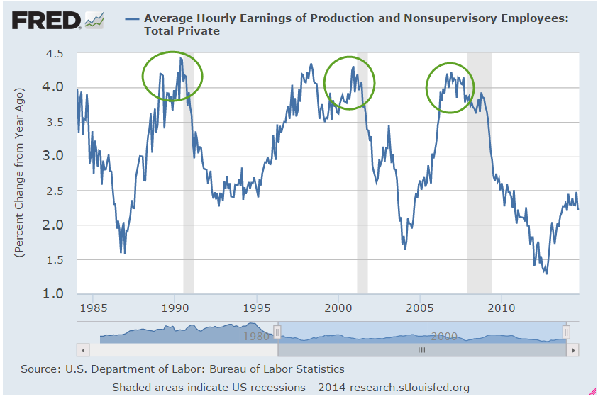
Strong wage growth had preceded the past three recessions.  Since this past recession, wage growth had fallen and stayed persistently low, causing discontent among frustrated voters.  Many workers were barely keeping up with inflation.

Voters were like the shade tree mechanics of George’s youth.  To adjust a carburetor, turn the screw this way or that way, trying to find the position where the engine idle sounded the smoothest.  It was a negotiation of sorts between air and gas.  Every two years, voters turned the political adjustment screw and waited to see if it made a difference.

Sales, Savings and Volatility

August 17, 2014

This week I’ll take a look at the latest retail sales figures, a less publicized volatility indicator, a comparison of BLS projections of the Labor Force Participation Rate, and the adding up of personal savings.

**********************

Retail Sales

Two economic reports which have a major influence on the market’s mood are the monthly employment and retail sales reports.  After a disappointing but healthy employment report this month, July’s retail sales numbers were disappointing, showing no growth for the second month in a row.  The year-over-year growth is 3.7%, which, after inflation, is about 1.5% real growth.  Excluding auto sales (blue line in the graph below), sales growth is 3.1, or about 1% real growth, the same as population growth.

As we can see in the graph below, the growth in auto sales has kicked in an additional 1/2% in growth during this recovery period. Total growth has been weakening for the past two years despite strong growth in auto sales, a sign of an underlying lack of consumer power.

Real disposable income rebounded in the first six months of this year after negative growth in the last half of 2013 but there does not seem to be a corresponding surge in sales.

*****************************

Labor Force Projections

While we are on the subject of telling the future…

All we need are 8 million more workers in the next two years to meet Labor Force projections made in 2007 by the Bureau of Labor Statistics (BLS).   8 million / 24 months = 300,000 a month net jobs gained. Hmmm…probably not.  In 2007, the BLS forecast slowing growth in the labor force in the decade 2006 – 2016.  Turned out it was a lot slower. Estimates then for 2016 projected a total of 164 million employed and unemployed.  In July 2014, the BLS put the current figure at 156 million employed.  The Great, or at least Big, Recession caused the BLS to revise their forecast a number of times.  The current estimate has a target date of 2022 to hit the magic 164 million.  In other words, we are 6 years behind schedule.

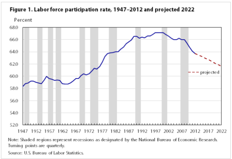
The Participation Rate is the ratio of the Civilian Labor Force to the Civilian Non-Institutional Population aged 16 and above.  The equation might be written:  (E + UI) / A = PR, where E = Employed, UI = Unemployed and Actively Looking for Work, and A = people older than 16 who are not in the military or in prison or in some institution that would prevent them from making a choice whether to work or not.  As people – the A divisor in the equation – live longer, the participation rate gets lower.  It ain’t rocket science, it’s math, as baseball legend Yogi Berra might have said.

The Participation Rate started rising in the 1970s as more women entered the work force, then peaked in the years 1997 – 2000.  Prior to the recession of 2001, the pattern of the participation rate was predictable, declining during an economic downturn, then rising again as the economy recovered.  The recovery after the recession of 2001 was different.  The rate continued to decline even as the economy strengthened.

In 2007, the BLS expected further declines in the rate from a historically high 67% in 2000 to 65.5% in 2016.  In 2012, the rate stood at 63.7%.  Current projections from the BLS estimate that the rate will drop to 61.6% by 2022.

Much of the decline in the participation rate was attributed to demographic causes in the 2007 BLS projections:

“Age, sex, race, and ethnicity are among the main factors responsible for the changes in the labor force participation rate.” (Pg. 38)

Comparing estimates by some smart and well trained people over a number of years should remind us that it is extremely difficult to predict the future.  We may mislead ourselves into thinking that we are better than average predictors.  Our jobs may seem fairly secure until they are not; a 5 year CD will get about 5 – 6% until it doesn’t; the stock market will sell for about 15x earnings until it doesn’t; bonds are safe until they’re not.

The richest people got rich and stay rich because they know how unpredictable the world really is.  They hire managers to shield them – hopefully – from that unpredictability.  They fund political campaigns to provide additional insurance against the willy-nilly of public policy.  They fight for government subsidies to provide a safety cushion, to offset portfolio losses and mitigate risk.  What do many of us who are not so rich do to insure ourselves against volatility?  Put our money in a safe place like a savings account or CD.  In real purchasing power, that costs us 1 – 2%, the difference between inflation and the paltry interest rate paid on those insured accounts.  In addition, we can pay a hidden “insurance” fee of 4% in foregone returns by being out of the stock and bond markets.  We stay safe – and not-rich.  Rich people manage to stay safe – and rich – by not doing what the not-rich people do to stay safe.  Yogi Berra couldn’t have said it better.

***************************

China

For you China watchers out there, Bloomberg economists have compiled a monetary index from several key factors of monetary policy.  After hovering near decade lows, China’s central bank has considerably loosened lending in the past two months.  The chart shows the huge influx of monetary stimulus that China provided in 2009 and 2010 as the developed world tried to climb up out of the pit of the world wide financial crisis.

The tug of war in China is the same as in many countries.  Politicians want growth.  Central banks worry about inflation.  The rise in this index indicates that the central bank is either 1) bowing to political pressure, or 2) feels that inflationary pressures are low enough that they can afford to loosen the monetary reins.  As is often the case with monetary policy, it is probably some combination of the two.

**************************
Personal Savings Rate

Over the past two decades, economists have noted the low level of savings by American workers.  While economists debate methodologies and implications, politicians crank up their spin machines. More conservative politicians cite the low savings rate as an indication of a lack of personal responsibilty.  As workers become ever more dependent on government programs, they do not feel the need to save.  Over on the left side of the political aisle, liberals cite the low savings rate as a sign of the growing divide between the middle class and the rich.  Many families can not afford to save for a house, or their retirement, or put aside money for their children’s education.  We need more programs to correct the economic inequalities, they say.

While there might be some truth in both viewpoints, the plain fact is that the Personal Savings Rate doesn’t measure savings as most of us understand the term.  A more accurate title for what the government calls a savings rate would be “Delayed Consumption Rate.”  The methodology used by the Dept. of Commerce counts whatever is not spent by consumers as savings.  “To consume now or consume later, that is the question.”
If a worker puts money into a 401K each month, the employer’s matching contribution is not counted.  If a consumer saves up for a down payment for a house, that is included in savings.  When she takes money out of savings to buy the house, that is a negative savings.  The house has no value in the “savings” calculation.  Many investors have a large part of their savings in mutual funds through personal accounts and 401K plans at work.  Capital gains in those funds are not counted as savings.  (Federal Reserve paper) In short, it is a poor metric of the aggregate behavior of consumers.  Some economists will point out that the savings rate indicates a level of demand that consumers have in reserve but because a significant portion of saved income is not counted, it fails to properly account for that either.

************************

Volatility – A section for mid-term traders

No one can accurately predict the future but we can examine the guesses that people make about the future.  In his 2004 book The Wisdom of Crowds (excerpt here) James Surowiecki relates a number of studies in which people are asked to guess answers to intractable problems, like how many jelly beans are in a jar.  As would be expected, respondents rarely get it right.  The surprising find was that the average of guesses was remarkably close to the correct answer.

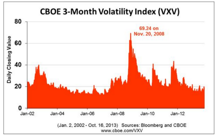
Through the use of option contracts, millions of traders try to guess the market’s direction or insure themselves against a change in price trend.  A popular and often quoted gauge of the fear in the market is the VIX, a statistical measure of the implied volatility of option contracts that expire in the next thirty days.  When this fear index is below 20, it indicates that traders do not anticipate abrupt changes in stock prices.

Less mentioned is the 3 month fear index, VXV (comparison from CBOE). Because of its longer time horizon, it might more properly be called a worry index.  Many casual investors have neither the time, inclination or resources to digest and analyze the many economic and financial conditions that impact the market.  So what could be easier than taking a cue from traders preoccupied with the market?  Below is a historical chart of the 3 month volatility index.

Historically, when this gauge has crossed above the 20 mark for a couple of weeks, it indicates an elevated state of worry among traders.  The 48 month or 4 year average of the index is 19.76.  Currently, we are at a particularly tranquil level of 14.42.

When traders get really spooked, the 10 day average of this anxiety index will climb to nosebleed heights as it did during the financial crisis.  As the market calms down, the average will drift back into the 20s range, an opportunity for a mid-term trader to get cautiously back into the water, alert for any reversal of sentiment.

*********************

Takeaways

Retail sales have flat-lined this summer but y-o-y gains are respectable.  So-so income growth constrains many consumers.  The 3 month volatility index is a quick and dirty summary of the mid-term anxiety level of traders.  A comparison of BLS labor force projections shows the difficulty of making accurate predictions.  The personal savings rate under-counts savings.