Home Sweet Asset

April 3, 2016

Normally we do not include the value of our home in our portfolio.  A few weeks ago I suggested an alternative: including a home value based on it’s imputed cash flows.  Let’s look again at the implied income and expense flows from owning a home as a way of building a budget.  The Bureau of Labor Statistics and the Census Bureau take that flow approach, called Owner Equivalent Rent (OER), when constructing the CPI, and homeowners are well advised to adopt this perspective.  Why?

1) By regarding the house as an asset generating flows, it may provide some emotional detachment from the house, a sometimes difficult chore when a couple has lived in the home a long time, perhaps raised a family, etc.

2) It focuses a homeowner on the monthly income and rent expense connected with their home ownership.  It asks a homeowner to visualize themselves separately as asset owner and home renter. It is easy for homeowners to think of a mortgage free home as an almost free place to live. It’s not.

3) Provides realistic budgeting for older people on fixed incomes.  Some financial planners recommend spending no more than 25% of income on housing in order to leave room for rising medical expenses.  Some use a 33% figure if most of the income is net and not taxed.  For this article, I’ll compromise and use 30% as a recommended housing share of the budget.

A fully paid for home that would rent for $2000 is an investment that generates an implied $1400 in income per month, using a 70% net multiplier as I did in my previous post. Our net expense of $600 a month includes home insurance, property taxes, maintenance and minor repairs, as well as an allowance for periodic repairs like a new roof, and capital improvements.

Using the 30% rule, some people might think that their housing expense was within prudent budget guidelines as long as their income was more than $2000 a month.  $600 / $2000 is 30%.

However, let’s separate the roles involved in home ownership.  The renter pays $2000 a month, implying that this renter needs $6700 a month in income to stay within the recommended 30% share of the budget for housing expense.  The owner receives $1400 in net income a month, leaving a balance of $5300 in income needed to stay within the 30% budget recommendation. $6700 – $1400 = $5300.  Some readers may be scratching their heads.  Using the first method – actual expenses – a homeowner would need only $2000 per month income to stay within recommended guidelines.  Using the second method of separating the owner and renter roles, a homeowner would need $5300 a month income. A huge difference!

Let’s say that a couple is getting $5000 a month from Social Security, pension and other investment income.  Using the second method, this couple is $300 below the prudent budget recommendation of 30% for housing expense.  That couple may make no changes but now they understand that they have chosen to spend a bit more on their housing needs each month.  If – or when – rising medical expenses prompt them to revisit their budget choices, they can do so in the full understanding that their housing expenses have been over the recommended budget share.

This second method may prompt us to look anew at our choices.  Depending on our needs and changing circumstances, do we want to spend $2000 a month for a house to live in?  Perhaps we no longer need as much space.  Perhaps we could get a suitable apartment or townhome for $1400?  Should we move?  Perhaps yes, perhaps no.  Separating the dual roles of owner and renter involved in owning a home, we can make ourselves more aware of the implied cost of our decision to stay in the house.  A house may be a treasure house of memories but it is also an asset.  Assets must generate cash flows which cover living expenses that grow with the passage of time.

/////////////////////

The Thrivers and Strugglers

“Bravo to MacKenzie. When she was born, she chose married, white, well-educated parents who live in an affluent, mostly white neighborhood with great public schools.”

In a recent report published by the Federal Reserve Bank at St. Louis, the authors found that four demographic characteristics were the chief factors for financial wealth and security:  1) age; 2) birth year; 3) education; 4) race/ethnicity.

While it is no surpise that our wealth grows as we age, readers might be puzzled to learn that the year of our birth has an important influence on our accumulation of wealth.  Those who came of age during the depression had a harder time building wealth than those who reached adulthood in the 1980s.

Ingenuity, dedication, persistence and effort are determinants of wealth but we should not forget that the leading causes of wealth accumulation in a large population are mostly accidental.  It is a humbling realization that should make all of us hate statistics!  We want to believe that success is all due to our hard work, genius and determination.

//////////////////////

Employment

March’s job gains of 215K met expectations, while the unemployment rate ticked up a notch, an encouraging sign.  Those on the margins are feeling more confident about finding a job and have started actively searching for work.  The number of discouraged workers has declined 20% in the past 12 months.

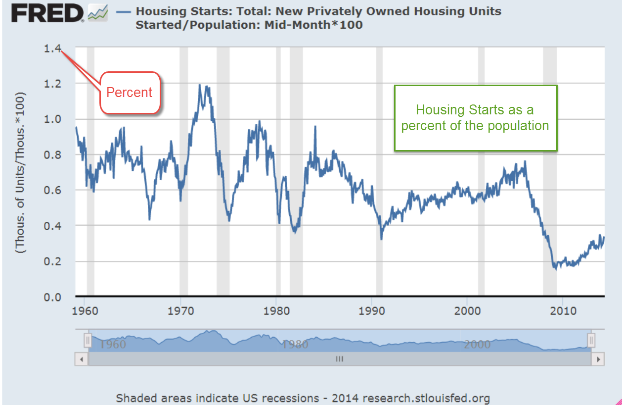
Employers continue to add construction jobs, but as a percent of the workforce there is more healing still to be done.

The y-o-y growth in the core workforce, aged 25-54, continues to edge up toward 1.5%, a healthly level it last cleared in  the spring of last year.

The Labor Market Conditions Index (LMCI) maintained by the Federal Reserve is a composite of about 20 employment indicators that the Fed uses to gauge the overall strength and direction of the labor market.  The March reading won’t be available for a couple of weeks, but the February reading was -2.4%.

Inflation is below the Fed’s 2% target, wage gains have been minimal, and although employment gains remain relatively strong, there is little evidence to compel Chairwoman Yellen and the rate setting committee (FOMC) to maintain a hard line on raising interest rates in the coming months.  I’m sure Ms. Yellen would like to get Fed Funds rate to at least a .5% (.62% actual) level so that the Fed has some ability to lower them again if the economy shows signs of weakening.  Earlier this year the goal was to have at least a 1% rate by the end of 2016 but the data has lessened the urgency in reaching that goal.

ISM will release the rest of their Purchasing Manager’s Index next week and I will update the CWPI in my next blog.  I will be looking for an uptick in new orders and employment.  Manufacturing lost almost 30,000 jobs this past month – most of that loss in durable goods.  Let’s see if the services sector can offset that weakness.

///////////////////////////

Company Earnings

Quarterly earnings season is soon upon us and Fact Set reports that earnings for the first quarter are estimated to be down almost 10% from this quarter a year ago.  The ten year chart of forward earnings estimates and the price of the SP500 indicates that prices overestimated earnings growth and has traded in a range for the past year.  March’s closing price was still below the close of February 2015.  Falling oil prices have taken a shark bite out of earnings for the big oil giants like Exxon and Chevron and this has dragged down earnings growth for the entire SP500 index.

Building Or Not

March 13, 2016

There are some upcoming changes to claiming rules for Social Security (SS) that take effect at the end of April.  A few weeks ago, Vanguard posted an article explaining some of the changes.

1) The end of “file and suspend,” the strategy where one half of a married couple, “John” we’ll call him, files for SS, then requests that those benefits be suspended.  The spouse, “Mary”, claims a spousal benefit while John’s benefits continue to grow at 8% per year until John is 70 years old.

2) The end of the “restricted application” strategy that allowed a person between the ages of 62 and 70 to collect benefits based on either their work history or their spouse’s history.  This allowed married couples to suspend taking benefits so that they could grow as under the file and suspend strategy.

////////////////////

You Didn’t Build That
In a 2012 campaign speech, President Obama infamously said, “If you’ve got a business — you didn’t build that. Somebody else made that happen.”

With the aid of teleprompters (only $2700) Mr. Obama  is a stirring orator, unlike his predecessor, Mr. Bush, who struggled with pronunciation, cadence and tone.  In contrast to his sweeping rhetoric, impromptu remarks by Mr. Obama are notoriously equivocal or inartful.  This remark was one of those.  Later on in the speech, Obama clarified his sentiments, “we succeed because of our individual initiative, but also because we do things together.”

In the 2012 election, Republican nominee Mitt Romney used Obama’s own words against him many times.  Many small business start-ups fail and when they do, the bank does not say, “you don’t need to pay your business loan back.  Somebody else made that failure happen.”  In Obama’s philosophy, failure is our personal responsibility but success is not?  It doesn’t play well in the small business community.

In response to February’s job report released last week, Mr. Obama is quite willing to take credit for the jobs created in the past seven years: “the plans that we have put in place to grow the economy have worked.” (Video and transcript) Mr. Obama doesn’t specify what plans.  The President and Congress, Democratic and Republican, have failed to enact fiscal policies that will help American businesses grow.  These leaders, these lifeguards of the economy, can not swim.  The Federal Reserve has had to implement extraordinary monetary policy to keep Americans from drowning.  0% interest rates for SEVEN years and $4 trillion of asset purchases by the Fed have reinflated the stock market and housing prices, the life raft of wealth for most Americans.

A fundamental theme of many elections is “It’s the economy, stupid,” a core mantra of the 1992 Clinton campaign coined by strategist James Carville.   Race and bigotry, defense and security play a part in a candidate’s appeal, but jobs, wages, benefits and taxes motivate voters to pull the lever in a voting booth.  The two outsider candidates, Bernie Sanders and Donald Trump, play to these economic concerns by promising jobs, or free college and medical care. Both candidates have been accused of being unrealistic and dangerous.

Once in office, most Presidents come to realize the reduced power they have in a Constitutional framework of checks and balances.  Each President must cooperate with a Congress easily swayed by lobbying interests, and fifty state legislatures with varying priorities and interests.

FDR exerted king-like powers during the multiple tenures of his Presidency thanks to the unprecedented majorities in both the House and Senate during the 1930s.  In the 1937-38 session, the Senate was dominated by 76 Democrats out of 100 members.  334 Democrats overwhelmed the 88 Republican members in the House.  During those years, the Supreme Court radically shifted the permissible Constitutional role of the Federal government in our lives.  The four generations that have lived since those policies were enacted continue to struggle with the social and financial consequences of those policies.

We are unlikely to repeat the lopsided majorities of that era simply because we recognize that unrestrained legislative power is dangerous and unhealthy for both our society and economy.  The Parliamentary systems of other developed countries allow a minority of citizens to have it their way, to dominate the policy choices of the majority.  The republican (small ‘r’) and federalist values embedded in the U.S. Constitution make it so much more difficult for a group of American citizens to get their way.  While this is often a source of frustration to policy advocates, we don’t veer off center as easily as other countries.

Focused on the 2016 election, voters may not notice the creeping dangers implicit in the extraordinary monetary measures and debt accumulation of the past twenty years.

Still Worried

November 1, 2015

Today is the day that U.S. readers fall back.  Let’s hope it’s the only thing that falls back!

Eight years ago, in October 2007, the SP500 index reached a pre-recession high of 1550. After this month’s 8% recovery the index stands at 2079, more than a third above that long ago high.  A decade long chart of the SP500 shows the inflection points of sentiment.  We can compare two averages to understand the shifts in investor confidence.  A three month average, one quarter of a year, captures short term concerns and hesitations.  A one year average reflects doubts or optimisms that have strengthened over time.  The crossing of one average above or below the other gives us a signal that a change may be coming.  Concerns may be temporary – or not.

After falling below the 12 month average, the 3 month average strained and groaned to pull its chin above that long average, notching five consecutive weekly gains.  Both China and the EU central banks have announced plans for lower interest rates or QE to spur their economies.  Oil prices continued to bounce around under the $50 mark.  OPEC suppliers announced they could not agree on production cuts.  Fearing a continuing oversupply of crude, oil prices fell 4 – 5%.  Then came the news that the number of oil rigs in the U.S. had fallen.  Prices went back up.

Commodities and mining stocks remain under pressure.  After falling over 18% in September, mining stocks gained back most of those losses in the first two weeks of October, then fell back in the last half of this month, closing the month with a 3% gain.  15 to 20% gains and losses in a sector during a month looks like so much scurrying and confusion.

Emerging market indexes lost ground this past week, slipping more than 4%.  Worries of a global recession continue to haunt various markets.  For large and medium U.S. companies, a slowdown in European and Asian markets is sure to have a negative effect on the bottom line.

The first estimate of 3rd quarter GDP growth was a paltry 1.5%, far below the 3.9% annual rate of the 2nd quarter.  Two-thirds of the SP500 companies have reported earnings for the 3rd quarter and FactSet estimates a decline of 2.2% for the quarter, the second consecutive quarter of earnings declines.

***********************

The Causes of Depression

The economic kind, not the emotional and psychological variety.  Economics history buffs will enjoy David Stockman’s critique of the extraordinary amount of monetary easing under former Fed chairman Ben Bernanke.  As President Reagan’s budget director, Stockman was at the forefront of supply side economics, a theory which promised an answer to the stagflation of the 1970s that drove many to question the assumptions and conclusions of Keynesian economics.

At first a champion of this new approach to economic policy making, Stockman grew disillusioned and later coined the term “voodoo economics” to describe the contradictory thinking of his boss and others in the Republican Party who stuck by their beliefs in supply side economics in spite of the evidence that these policies generated large budget deficits and erratic economic cycles.

In 2010, Stockman penned an editorial  that held some in the Republican Party, his party, culpable for the 2008 fiscal crisis.  He understands that politicians and policy makers become welded to their ideological platforms, disregarding any input that might upset their model of the world.

For those who have a bit of time, an Atlantic magazine December 1981 an article acquainted readers with David Stockman in his first year as budget director.  The budget process seems as broken today as it was 35 years ago when Stockman assumed the task of constructing a Federal budget.

 These “internal mysteries” of the budget process were not dwelt upon by either side, for there was no point in confusing the clear lines of political debate with a much deeper and unanswerable question: Does anyone truly understand, much less control, the dynamics of the federal budget intertwined with the mysteries of the national economy?

Stockman understands the political gamesmanship that permeates Washington.  He criticizes Bernanke’s analysis of the 2008 Great Recession as well as the 1930s Great Depression. Faulty analysis produces faulty remedies. Stockman goes still further, finding fault with Milton Friedman’s monetary analysis of the causes of the Great Depression.  In a 1963 study titled A Monetary History of the United States Friedman and co-author Anna Schwartz found that monetary actions by the Federal Reserve deepened and lengthened the 1930s Depression.  Friedman became the leading spokesman of monetarism in the late 20th century, the thinking that governments can more effectively guide a national economy by adjusting the money supply rather than employing an ever changing regime of fiscal policies.

Students of the great debate of the past 100 years – bottom up or top down? – will enjoy Stockman’s take on the matter.

Holding Pattern

September 20, 2015

The big news this week was the decision by the Fed to not raise interest rates this month.  Big mistake.  The Fed’s decision signaled a lack of confidence in the global economy.  Are we to believe that the continuing strength of the American economy is so weak that it can not weather even a 1/4% interest rate increase?

Message received.  When the news was announced on Thursday, the initial reaction was good.  Yaay!  no rate increase.  Then, the reality sunk in.  Does the Fed know something that the rest of us don’t? The buyers went to the back of the bus.  The sellers started driving the bus.  Pessimism wiped out the gains in the early part of the week and ended the week down 7/10%.  When in doubt, traders get out.

There are many aspects of the labor market.  The Fed crafts a composite of over 20 factors, called the Labor Market Conditions Index (LMCI).  The latest reading was released on September 9th, a week before this month’s Fed meeting.  This may have contributed to the caution in the Fed’s decision making.  The overall labor market has still not fully recovered from the downturn this past spring.

****************************
Automation

Will your job become automated?  In this fast morphing economy, the demand for a particular skill set can change quickly.  Younger people, whether working or still in school, need to focus on developing transferable skills.   Here’s a list of the nine criteria that some researchers determined were important to keeping a job from being automated: “social perceptiveness, negotiation, persuasion, assisting and caring for others, originality, fine arts, finger dexterity, manual dexterity and the need to work in a cramped work space.”

When the first Boomers were born at the end of World War II, 16% of the workforce was employed in agriculture.  Millions of agricultural jobs have been lost in the past 70 years. Now it is less than 2%. (USDA source)

Computerization has led to the loss of millions of clerical and accounting jobs in the back offices of businesses throughout this country. Despite those job losses of the past 25 years, there are almost twice as many professional and business employees now as there were in 1990 (Source )

In contrast, construction employment is about the same as it was 20 years ago – an example of an industry that boomed and busted in the past two decades.  Despite that lack of growth, construction employment is still almost twice what it was in the go-go years of the 1960s. (Source)

Despite all these job losses due to automation and more efficient production methods, there are 350% more people working now (140 million) than there were at the end of WW2 (40 million). (Source)

Those who get left behind are those who have a narrow set of skills.

*************************
Labor Market Analysis

Each August the Federal Reserve hosts an economic summit for central bankers, economists and academics.  In 2014, Fed chair woman Janet Yellen commented on several aspects of the labor market:

Labor force participation peaked in early 2000, so its decline began well before the Great Recession. A portion of that decline clearly relates to the aging of the baby boom generation. But the pace of decline accelerated with the recession. As an accounting matter, the drop in the participation rate since 2008 can be attributed to increases in four factors: retirement, disability, school enrollment, and other reasons, including worker discouragement.

As Yellen noted, some changes were structural, some cyclical:
Over the past several years, wage inflation, as measured by several different indexes, has averaged about 2 percent, and there has been little evidence of any broad-based acceleration in either wages or compensation. Indeed, in real terms, wages have been about flat, growing less than labor productivity.

Ms. Yellen agrees that the headline unemployment rate, the U-3 rate, does not reflect current labor market conditions:  “the recent behavior of both nominal and real wages point to weaker labor market conditions than would be indicated by the current unemployment rate.

Since unemployment peaked at 25% during the Great Depression in the 1930s there has been an ongoing debate about unemployment during recessions.  Why don’t employees simply offer to work for less when the economy starts slowing down? Yellen offered some insights [my comments in brackets below]:

the sluggish pace of nominal [current dollars] and real [inflation-adjusted] wage growth in recent years may reflect the phenomenon of ‘pent-up wage deflation.’ The evidence suggests that many firms faced significant constraints in lowering compensation during the recession and the earlier part of the recovery because of ‘downward nominal wage rigidity’–namely, an inability or unwillingness on the part of firms to cut nominal wages. To the extent that firms faced limits in reducing real and nominal wages when the labor market was exceptionally weak, they may find that now they do not need to raise wages to attract qualified workers. As a result, wages might rise relatively slowly as the labor market strengthens. If pent-up wage deflation is holding down wage growth, the current very moderate wage growth could be a misleading signal of the degree of remaining slack. Further, wages could begin to rise at a noticeably more rapid pace once pent-up wage deflation has been absorbed.”

Steady As She Goes

March 22, 2015

Monetary Policy

The FOMC is a committee of Federal Reserve members who meet every six weeks to determine the course of monetary policy.  A statement issued at the end of each two day meeting is carefully parsed by traders in an orgy of exegesis.  And thus it was so this past week.  Recent statements by the Fed included the word “patient” as in low inflation and some lingering weaknesses in the labor market allow us to take a patient approach with monetary policy.  If the Fed removed the word patient, then it was a good bet that they would start raising rates at their mid June meeting.  By the end of the year, the thinking was, the benchmark Fed funds rate could be 1%-1.25%.

So here’s what happened while you were at work, or at lunch or picking up the kids on Wednesday afternoon when the Fed meeting concluded. The initial reaction was negative, or at least that’s how the HFT (high frequency) algorithms parsed the Fed’s statement.  “Patient” was gone.  Sell, sell, sell. Then some human traders noticed that the Fed was also saying that they did not have to be impatient either – the perfect neutral stance.  Buy, buy, buy.  The SP500 jumped 1.5% in a few minutes.  The neutral stance of  the Fed caused many to revise their estimates of the Fed rate at the end of the year to .75% or less.  The broad market index ended the week at the same level as it was when the month began.  Volatility as measured by the VIX is rather low but there has been a lot of  positioning since Christmas and a net gain of only 1% in those three months.

*********************

Earnings Recession


The analytics firm FactSet projects a year-over-year decline in the earnings of the SP500 companies for this first quarter of 2015.  Here is a good review of the historical response of the stock market to earnings recessions, defined as two quarters of year-over-year declines in the composite earnings of the SP500.

***********************

Oil

Oil is an international commodity that trades on world markets in U.S. dollars.  A prudent strategy for countries which are net importers of oil is to stock up on dollars to pay for its short term oil needs.   As the demand for dollars climbs so does its price in other currencies, a self-reinforcing mechanism.  Half of the drop in the price of oil is due merely to the appreciation of the dollar, which has spiked some 25% since the beginning of the year.

For decades, many in academia and government have advocated the adoption of an international currency called the SDR, already in use by the International Money Fund.   Here is an article from last May, before the price of oil started its slide.  The dollar is the latest in a series of reserve currencies over the past 500 years and has been the dominant currency for almost 100 years (History here). The reliance on one country’s currency works – until it begins to cause more problems than it solves.  The  largest producer and consumer of oil, Saudi Arabia and the U.S., have formed a decades long agreement to price oil in U.S. dollars, binding the rest of the world to the movements in the U.S. dollar.The recent volatility in the dollar in threatening the economic stability of many nations, who are increasing their calls for a change in international monetary policy.

***********************

Sticky CPI

In a survey of newspaper articles, inflation was mentioned more than unemployment or productivity.  In the U.S., inflation is often measured by the Consumer Price Index (CPI).  A subset of that measure is called the core CPI and excludes more volatile food and energy items to arrive at a fundamental trend in inflation.  (IMF primer on inflation ) Critics of the core CPI point out that food and energy items are the most frequent purchases that consumers make and have a fundamental effect on the economic well being of U.S. households.  Responding to some of the inherent weaknesses in the methodology of the CPI, the Atlanta branch of the Federal Reserve began development of an alternative measure of inflation – a “sticky” CPI. (History)  This metric gives a statistical weight to the components of the CPI by how much prices change for each component.  The Atlanta Fed has an interactive graph that charts both the sticky measure and a more volatile, or flexible CPI that is similar to the conventional CPI.  The sticky CPI tends to measure expectations of future changes in inflation and moves rather slowly.

Over a half century, the clearest trend is the closing of the gap between the regular CPI and the sticky CPI.

When we compare all three measures, core, sticky and regular CPI, we see that the sticky CPI is usually above the core CPI.  January’s readings are 2.06% for the sticky index, 1.64% for the core index and -.19% for the headline CPI index.

A private project called Price Stats goes through the internet comparing prices on billions of items.(WSJ blog article here)  This data is more timely and shows an uptick in core inflation that is approaching 2%, the Federal Reserve’s target rate.  When asked why the Fed uses 2%, chair Janet Yellen answered that inflation indexes do not capture improvements in products, only prices, so they tend to overstate inflation as a matter of design and practical data gathering.  Secondly, the 2% mark gives the Fed a statistical cushion so that they are able to take appropriate monetary steps to avoid deflation.

Why is deflation a bad thing?  In answering this question, we discover the true benefit of the core CPI.  Food and energy are regularly consumed.  Demand for these goods is relatively “sticky”.  A family may change what types of foods it buys in response to price changes but it is going to buy food. Deflation in these core purchases can be a good thing as it takes less of a bite out of the average household’s wallet.

On the other hand, deflation in less frequently purchased goods, which the core CPI tracks, is not good because it leads to a self-perpetuating cycle in which consumers delay making purchases in the expectation that tomorrow’s price will be lower than today’s price.  If I expect that the price of an iPhone will be lower next week, how likely am I to buy one this week?  As consumers delay purchases, suppliers lower prices even more to move their goods.  Seeing the price competition among vendors, consumers are even more likely to delay purchases, waiting for prices to come down even further.  As sales drop, vendors and manufacturers begin to layoff employees.  Lower prices no longer entice consumers who become concerned about keeping their jobs and purchase only what they need.

***********************
Indicators

The Conference Board, a business association, released their monthly index of Leading Indicators this week but it has a spotty history of forecasting trends. Doug Short puts together a nice snapshot of the Big Four indicators, Employment, Real (inflation-adjusted) Sales, Industrial Production, and Real Income.

How Much Is That Doggie In the Window?

June 22, 2014

This week I’ll look at interest rates and various models of evaluating both the stock market and housing.

*****************

GDP Growth Revised

This past Monday, the International Monetary Fund (IMF) cut estimates for this year’s economic growth in the U.S. to 2% from 2.8%.  IMF cited a number of headwinds: the severe winter, weakness in housing, some fragility in the labor market.  It recommends that the central bank keep rates low through 2017.  Expectations were that the Federal Reserve would begin raising interest rates in mid 2015.  Some recommendations in the report will be met with antipathy or a polite “thanks for letting us know”: raising the minimum wage and gasoline taxes.

******************

Fed Don’t Fail Me Now

As expected, the Federal Reserve decided to leave the target interest rate at the extremely low range of 0% to .25% that it has held in place since the beginning of 2009.  Congress has given the Fed a dual mandate:  keep inflation reasonable and promote full employment.  It is this second half of the mandate that presents some problems as the FOMC looks into their crystal ball.  The Labor Force Participation Rate is the percentage of those working to those old enough to work.  It has declined from 66% at the beginning of the recession to less than 63% today.

As economic conditions improve and job prospects brighten, how many of those who have dropped out of the labor force will return?  If workers return to the labor force, actively seeking work, that increased supply of labor will naturally curb wage increases and reduce upward pressure on inflation.  However, if the decline in the participation rate is more or less permanent for several years to a decade, then a stronger economy will create more demand for workers, who can demand more money for their labor, which will contribute to inflation.

**********************

401K Retirement Plans

The Financial Times reported projections  of negative cash flows in 401K plans by 2016 as boomers convert their pension plans to IRAs when they retire.  Retirees tend to have a much more conservative stock/bond allocation and may force institutional money managers to liquidate some equities to meet the outgoing cash flows.  An ominous speculation at the end of the article is that regulations could be put in place to slow the conversion of 401Ks to IRAs.  Whenever the finance industry needs a friend in Washington, they can be sure to find one.

*********************

Stock Market Valuation

It has been 32 months without a 10% correction in the SP500 market index.  The post World War 2 average is 18 months. Is the stock market overvalued?  I will review a common metric of value and develop an alternative model of long-term value.

Probably the most widely used metric of stock valuation is the Price/Earnings, or PE, ratio.  If a stock sells for $100 and its annual earnings are $6, then the P/E ratio is 100/6, or a bit above 16.  The average PE ratio is 15.5 (Source).  Companies do not pay all of those earnings in the form of dividends to investors.  That is another metric, called the Price Dividend, or P/D ratio, that I wrote about last year.

Fact Set provides an analysis of the past quarter’s earnings of the SP500 companies, as well as projections of current  and next year’s earnings. Earnings growth estimates for this year range from 30% (yikes!) for the telecom sector to a bit over 3% for utilities. The health care sector tops estimates of revenue growth at about 8%, while the energy sector is projected to have negative growth.  The basic materials sector tops the 2015 list of earnings growth at 18% and the utilities sector again takes the bottom rung on the ladder with almost 4% growth.

The SP500 is priced at 15.6x forward 12 months earnings, which is above the five year and 10 year averages of less than 14x (Fact Set Report page)  but just about the 100 year average of 15.5.

Robert Shiller, a Yale economist and co-developer of the Case-Shiller housing index, uses a smoothing technique for calculating a Price Earnings ratio and makes his data spreadsheet available.  His team calculates the 10 year average of real, or inflation-adjusted, earnings and divides the inflation adjusted price of the SP500 by that average to arrive at a Cyclically Adjusted Price Earnings, or CAPE, ratio.

Using this methodology, the market’s CAPE  ratio is 25, above the 30 year ratio of 22.91 and the 50 year ratio of 19.57.  In 1996, the market was trading at this same ratio, prompting then Fed Chairman Alan Greenspan to make his infamous comment about “irrational exuberance.”  The market continued to climb till it reached a nosebleed CAPE ratio of 43 in early 2000.  It took another 7 months or so before the SP500 began its descent from 1485 to 900, a drop of 40%, over the next two years.  There is no automatic switch that flips when a market becomes overvalued.  People just get up from their seats and start to leave the theater.

In most decades, this methodology works well to arrive at a longer term perspective of the market’s price.  However, some argue that when severe downturns occur, this methodology continues to factor in the downturn’s impact long after it they have passed.  In 2008 and 2009, SP500 index annual earnings crashed from above $80 down to $60, a precipitous decline that is still factored into the ten year framework of the CAPE method.

So I took Mr. Shiller’s earnings figures and did some magic on them.  I took away most of the downturn in earnings during a 3 year period from 2008 – 2010.

Bye, bye earnings dive.  Hello, stagnating earnings.  The chart shows a slight downturn in earnings, then flat-lines in the pretend world of 2008 – 2010, where the steep recession never happened.

Instead of a deep crater formed in the markets by the financial panic in late 2008, the stock market slid downward over several years before rising again in early 2012.  Can you hear the soft sounds of flutes echoing in the mountain meadows of this pretend world?

Using this pretend data, I recalculated today’s CAPE ratio at 22, below the actual 25 CAPE ratio.  What should be the benchmark in this pretend world?  The 100 year average includes the Great Depression of the 1930s and World War 2, which naturally lowered PE ratios.  A 50 year average includes the Vietnam War and high inflation, particularly during the 1970s and early 1980s.  As such, it is less comparable to today’s environment marked by low inflation and the lack of major hostilities.

So, I ran a 30 year average of our pretend world, from 1984-2013, and calculated a 30 year average of 23, close to the real 30 year average of 22.9!  It shows the relatively small effect that even momentous events have on a long term average of the CAPE ratio, which is why Robert Shiller advocates its use to calculate value and establish a comparison benchmark within a longer time frame.  In the real world, the market’s CAPE ratio of 25 is above that 30 year average.

Let’s put aside the world of soft market landings and mountain meadows and look at what I call the time value of the market.  I picked January 1980, a point almost 35 years in the past, as a starting point.  Then I divided the SP500 index by the number of months that have passed since that starting point.  This gives me a ratio of value over time. If an investor buys into the market when its value is above a long-term average of that ratio, we can expect a lower long-term rate of return.

The 20 year average is 3.98, just a shade above the 20 year median of 3.91, meaning that the highs and lows of the average pretty much cancel out.  Note also that it is only in the past year that the market value has risen above the 20 year average of this ratio.

But we cannot look at a time value of any investment without considering inflation, which erodes value over time.  When we add the Time Value Ratio and the Consumer Price Index (CPI), we find that the current market is priced slightly lower than both the 20 year and 30 year averages.

Historically, as this ratio has risen more than 25 – 30% above its long-term average,  the market peaked.  Today’s ratio is just about average.

So, is the market overvalued?  Based on CAPE methodology, yes.  Fairly valued?  Based on expectations of earnings growth this year and next, yes.  Undervalued?  Probably not.

Common Sense recently published the best and worst 10 and 20 year returns on a 50/50 stock/bond portfolio mix.  This balanced approach had a 2 – 3% annualized gain even during the Depression years when the stock market lost 80 – 90% of its value.  It should be a reminder to all investors that trying to assess the true value of the stock market is perhaps less important than staying diversified.

************************

The P/E of Housing

Home builders broke ground on almost 1.1 million private residential units in April, a 13% increase over last year.  Called Housing Starts, the series includes both multi-family units and single family homes. The pace slowed a bit in May but still broke the 1 million mark.  As a percent of the population, we just aren’t building as many homes as we used to.

For most of us, our working years are about 60% of our lifespan.  Hopefully, our parents took care of our income needs for the first 20% of our lifespan. During our working years, we hope to save enough to generate a flow of income for the last 20% of our lifespan.  Those savings, which include private pensions and Social Security, are like a pool of water that we accumulate until we start turning on the spigot to start draining the pool.    We turn a stock or pool of savings into a flow of income.

The Bureau of Labor Statistics uses a metric called Owner Equivalent Rent (OER) in their calculation of the Consumer Price Index.  This concept treats a home as though it were generating a phantom income equivalent to the rents in that local real estate market.  We can use this concept to value a house.  The future flows from a stock can be used to generate an intrinsic current value for the house.

As an example:  a house which would generate a net $12000 a year in income, whether real or phantom, after taxes and other expenses, is worth about 16 times that net income, according to historical trends calculated by the ratings agency Moodys.  In this case, the house would be worth about $200K.

Coincidentally, this is the average P/E ratio of the stock market.  Historically, stocks have been valued so that the price of the company’s stock has been about 16 times the earnings flow from the company’s activities.  If a primary residence generates 6% in tax free income and 3% in appreciation, the total annual return on owning a house free and clear is more than the average annual return of the stock market.  The housing boom and bust may have given many younger people the impression that home ownership is a debt trap.  It may take a decade for the housing industry to recover from this perception.

**************************

Takeaways

The Fed is likely to keep interest rates low past mid-2015 but is watching the Labor Participation Rate for early indications that rising wage pressures will spur rising inflation.
The stock market is slightly overvalued or fairly valued depending on the metric one uses.
On average, a house has a value multipler that is similar to the stock market but generates a higher after tax income.

Next week I’ll take a look at some long term trends in education spending and tuition costs.

Earnings, Revenues and Retail Sales

April 20, 2014

You’re on a date with me, the pickin’s have been lush
And yet before this evenin’ is over you might give me the brush

Luck Be a Lady
from the play Guys and Dolls

Easy money

In opening remarks Tuesday at a Federal Reserve conference in Atlanta, Janet Yellen, head of the Fed, made the case that ongoing weakness in the global economy warranted support from central banks and that she did not anticipate full employment in the U.S. for another two years.  The Fed reported that the economies in all 12 Fed districts improved in March as consumers ventured out of their winter burrows. The stock market rose in each of the four trading days this week, but has still not risen to the level it opened at on Friday, April 11th, when the market dropped 2%.  Disappointing earnings reports restrained enthusiasm sparked by the prospect of continued easy monetary policy from the Fed.

**************************************

Earnings

On Tuesday, discount broker Charles Schwab reported a 58% increase in first quarter profits.  Trading volume was the highest in its history as many individual investors returned to the stock market.

In the tech sector, Intel and IBM reported declining revenues of 1% and 4% respectively.  The stock price of both companies is about the same as it was two years ago.  Intel is trying to transition from its traditional dominance in PC chips as sales of PCs continue to slow.  IBM is undergoing a similar transition from hardware – particularly mainframes – to business software.

Since early 2012, the Technology SPDR ETF,  a broad basket of tech stocks, is up almost 50%.  For an investor who does not have the time to research trends in a particular sector, particularly one as dynamic as the technology sector, buying a representative basket of the sector may be the safer choice.

American Express reported a first quarter drop in revenue of 4%, attributing most of the decline to small business and corporate spending.

Google reported an 8% drop in first quarter revenue from the fourth quarter.  Year over year, revenue rose 10% but investors have realized that the days of 20 – 40% annual revenue gains are probably over.  Since early March, the company’s stock has dropped 12%.

W.W. Grainger sells supplies, parts, equipment and tools to businesses.  Since 2009 revenues have risen almost 50% but sales growth has been meager since the middle of last year.  A few weeks ago, I noted the lack of growth in maintenance and repair employment.  Grainger’s lack of revenue growth and declining spending by businesses at American Express are disturbing indicators that there is a lack of confidence and investment in growth.

The industrial and financial megalith General Electric reported a year over year revenue increase of 2.2% but the company’s revenues have been fairly flat for four years and the stock price is almost 20% below its mid 2007 level.  GE is gradually shedding its financial businesses in order to focus on what it does best – making stuff, big stuff and small stuff.  With a dividend yield of 3.4%, this stock may be worth a more in depth look for investors who buy individual stocks and think that the company can make the transition.  As a side note:  in 2013, GE managed to defer $3.3 billion, or 85%, of its income tax liability, which will no doubt get some attention in the coming election cycle.  What won’t be mentioned is that GE paid over $8 billion in 2011 and 2012.

*************************************

Retail Sales and Household Debt

Retail sales were up a strong 1.1% in March, the most in two years.  Auto sales were particularly strong. Household debt is at the same level as it was in the 1st quarter of 2007 but has been slowly rising in the past year.  The years from the mid 1980s to the mid 2000s is often called the Great Moderation by many economists but the period is marked by an immoderate 8.6% annual growth rate in household debt.  Since the onset of the financial crisis and recession, households have jumped off that runaway train yet today’s levels still reflect a 34 year annualized growth rate of 7%.

With meager growth in personal income, it is unlikely that consumers can afford to rise to those heady and unsustainable growth rates in debt.  However, the percent of income needed to service that debt is at 34 year lows.  Growing consumer confidence and willingness to take on more debt may pull the economy out of the current lackluster growth.

*************************************

Margin Debt

A link on this blog is to the excellent work that Doug Short does.  In case you missed it, here are some graphs he presented on margin debt reported by the NY Stock Exchange, or the amount of money that investors have borrowed against their stock holdings.

I am not sure how reliable this indicator is.  Selling as margin debt starts to drop and buying as it starts rising again has mixed results.  The strategy would have kept a hypothetical investor out of the market during the market downturn in the early 2000s, back into the market in late 2003, out of the market in early 2008, and back into the market in July 2009.  So far, the timing looks great.  Since then, however, the rise and fall in margin debt has signaled some fake outs, so that an investor would have sold during a temporary market disruption, only to buy in later at a higher level.

Oddly enough, the last buy signal in February 2012 coincided with the Golden Cross in late January 2012.  The Golden Cross occurs when the 50 day moving average crosses above the 200 day moving average.

Retail, Housing, The Fed And More

Last week I pointed to several contradictory outlooks for sales in the upcoming holiday season.  Bill McBride at Calculated Risk has several charts on the import and export volume at the port of Los Angeles.  The import data indicates that businesses were buying goods in late summer and the fall in anticipation of a good holiday season.  Both Home Depot and Best Buy reported better than expected earnings on Tuesday but Best Buy’s sales were less than expected.  The company cited increasing pressure from online retailers.  E-Commerce continues to take an ever increasing share of the retail sales market.

Amazon is now making more money selling other vendors’ products than it does its own.  Vendors typically turn over much of the sales, shipping and billing process to Amazon.  Businesses, including mine, are increasingly turning to Amazon for parts or supplies.  Why?  Amazon has become an easy to search portal for so many vendors and the prices are competitive.  Why spend time searching the web for long discontinued parts when Amazon has already done that?  What is even more surprising is the enormous volume of third party items that Amazon now stocks and, surprisingly, the items are received from Amazon, not the vendor.

On Wednesday, the monthly report of retail sales showed a .4% month on month gain, causing analysts at Morgan Stanley to reverse their earlier dour opinion of the coming holiday season.  The year over year gain is at 4% but retailers that target lower income consumers are experiencing some difficulties.  J.C. Penney reported sales and earnings that were disappointing.  After an earlier upbeat report from the home improvement chain Home Depot, Lowe’s reported strong sales and earnings, confirming the continuing strength in this sector.  Later in the week, Target issued a disappointing earnings report.  Will the ongoing decline in gas prices leave working class families with enough extra cash in their wallets this Christmas season?  Wal-Mart, Target and J. C. Penney hope so.

**************************
[Revised to clarify the two separate housing indexes below]

 October’s housing market index reading of 54 from the National Assoc of Homebuilders indicated continuing strength in the new home market.  This index is a composite of factors, including sales, inventory, builder expectations and traffic.  The series, like the industrial reports, is indexed so that 50 is the neutral mark, indicating no net growth.  Although the overall index has declined from the summer peak, both sales and expectations are in the strong to robust growth.

The Federal Housing Finance Agency tracks an index of home prices (only).  Major markets on both the east and west coasts are still below the bubble peaks of 2005 – 2006.

From 1983 to 1999, the average house cost 13 to 15 years worth of rent.  This baseline is a good rule of thumb when pricing out houses.  In 2006, at the height of the housing bubble, houses were selling for 25 years worth of the average monthly rental.  Los Angeles experienced a much greater price inflation during the 2000s than either SF or NYC.  Although the nationwide economy is growing steadily but slowly, Los Angeles has responded to the strong growth in manufacturing throughout the country. Asking rents for industrial properties in L.A. are rocketing upward this year, accelerating from the strong three year growth and exceeding the price levels of 2007.

http://www.loopnet.com/xNet/MainSite/Tools/WidgetHTML.aspx?WidgetType=50&CountryCode=US&StateCode=CA&State=California&CityName=Los+Angeles&SiteID=1&TrendTypeID=2&PropertyTypeID=40&ListingType=LEASE&PropertyType=Industrial&TrendType=Asking%20Rent Available Office and Industrial property in the LA area is at multi-year lows.

http://www.loopnet.com/xNet/MainSite/Tools/WidgetHTML.aspx?WidgetType=50&CountryCode=US&StateCode=CA&State=California&CityName=Los+Angeles&SiteID=1&TrendTypeID=5&PropertyTypeID=80&ListingType=LEASE&PropertyType=Office&TrendType=No.%20of%20Spaces

Los Angeles, CA Market Trends

**************************

http://www.loopnet.com/xNet/MainSite/Tools/WidgetHTML.aspx?WidgetType=50&CountryCode=US&StateCode=CA&State=California&CityName=Los+Angeles&SiteID=1&TrendTypeID=5&PropertyTypeID=40&ListingType=LEASE&PropertyType=Industrial&TrendType=No.%20of%20Spaces
The Consumer Price Index released Wednesday showed a tiny decrease in inflation for the month.  The year over year change was 1.7%, indicating that demand at many levels is positive but weak so that there is little pressure on prices.  On Thursday, the Producer Price Index (PPI) confirmed that the supply chain is experiencing very low upward pressure.

***************************

The PMI Flash Index, a preview of the upcoming report on the manufacturing sector, confirmed the continuing growth in the manufacturing sector.

***************************

The Job Openings and Labor Turnover Survey (JOLTS) by the BLS was released on Friday.  Unlike the timeliness of the monthly Employment report, this one lags by a month but does provide a more comprehensive analysis of the growth or decline in the labor market.  The BLS surveys employers at the end of the month, September in this case, for job openings and layoffs.  A job opening can be full time, part time, seasonal or temporary so the data can be skewed by seasonality factors.  The longer term trend, though, is apparent.

It may be several more years before job openings reach the level attained during the tech boom of the late ’90s.  Like the gold fever of the mid-19th century, investors poured money into a lot of ventures with little more than a napkin sized business plan.  This pattern of bubble and bust is fairly typical when game changing technologies emerge.  The spread of the telegraph and railroads led to horrific recessions in the late 19th century, culminating in the depression of 1893-94.  The rise of radio in the 1920s prompted speculative fever that contributed mightily to the crash of 1929, setting the stage for the bad monetary policy and haphazaard fiscal policies that fed the depression of the 1930s.  In the 1960s, a rush of investment in airlines and war funding helped fuel a frenzy of speculation that crashed in 1970.

******************************

In Washington this week, the Senate voted to change the rules for Senate confirmation of most executive and judicial appointments, the so called “nuclear option” that requires only a majority vote for confirmation.  This modification of the filibuster rule should have been done ten years ago when then Democratic Senate Minority Leader Tom Daschle led filibusters to block many of George Bush’s appointments.  Since then, the Senate has grown ever more dysfunctional, incapable of even ordering pizza.  Under the elitist filibuster rules, each Senator could act like a despot or one of the “Knights who say ‘Nee’!” in the comic movie “Monty Python and the Holy Grail.”  A Senator representing 300,000 people in Wyoming could nix or delay an executive appointment – this in a country of over 300 million. Sounds a bit like England in the 1770s. A lot of people died in the Revolutionary War so that America would not be a country ruled by a despot, be it a king or a Senator.

*******************************

The rule change makes the confirmation of Janet Yellen as the next chair of the Federal Reserve a near certainty. In a speech at the Cato Institute’s Annual Monetary Conference, Charles Plosser, President of the Philadelphia branch of the Federal Reserve, made a good case for some restraint by the Federal Reserve – not in the amount of debt the Fed purchases but the type of debt:

“[The Federal Reserve’s] purchase [of] specific (non-Treasury) assets amounted to a form of credit allocation, which targets specific industries, sectors, or firms. These credit policies cross the boundary from monetary policy and venture into the realm of fiscal policy.”

Mr. Plosser would rather see politicians, not central bankers, decide which industries to favor through bailouts or loan purchases.  In a democratic republic like ours, if the politicians in Washington want to bailout banks or the housing sector, they can do so by issuing general debt obligations, Treasuries, which the Federal Reserve can buy.  Gridlock in Washington has prevented them from reaching any consensus about these policies, leaving it up to the Federal Reserve to act in their place, to make political decisions which compromises the neutral stance that a central bank should have.

Now, we might say that the result is the same so what’s the big deal?  Knowing that Fed chairman Ben Bernanke would come to the rescue has allowed politicians to not make difficult compromises.  Why should they?   If Congress does less, the Fed does more.  Because it can be so difficult to enact their agenda through the political process, Presidents and political parties turn to the Fed as the fourth branch of government.

Plosser also questions the dual target of both inflation and unemployment that the Fed has assumed as its mandate.  The law states that the Fed should enact monetary policy that is “commensurate” with the “long run potential to increase production.”  Since the recession began in 2008, the Fed has adopted a series of “QE” short term measures designed to decrease unemployment and Plosser’s view is that these are not part of the job description.  Plosser will be a voting member in 2014.  His vote of restraint is unlikely to hold much sway with Janet Yellen, who is ready to keep the cornucopia money machine flowing.

****************************

In the Wall St. Journal’s Washwire Blog, Elizabeth Williamson writes that the White House is conducting a self-assessment in the wake of the health-law launch, “recognizing that administration officials missed warning signs and put too much trust in their management practices.”   What on earth has given this administration any reason to trust their management practices?  Was it their management of the attack on the U.S. consulate in Benghazi in September 2012?  Or perhaps the “red line” that President Obama drew with Syria, promising a military response if Syria used chemical weapons against its own people?  Or the terribly mismanaged mortgage relief program, HAMP, that former Treasury Secretary Tim Geithner put in place?

This is only a partial list of the persistently poor management practices that have marked this administration.  It began with the poor preparation in advance of the March 2009 meeting with the nation’s largest banks, leading Obama and Geithner to offer generous terms to the banks when the banks would have accepted any terms in order to stay alive.  The crafting of the stimulus bill was an example of indecisive leadership and management at one of those rare times in history when both houses of Congress were controlled by the President’s party.  Using a basketball analogy, the administration blew a layup.

Now comes the news that the Obama administration wants to exempt some union health care plans from a “reinsurance tax” – about $63 per person per year – that all plans under the ACA health care law pay.  How will they do this?  By a carefully worded exemption that applies only to self-administered health plans.  A little background.  Many big companies self-insure and hire an administrator like Blue Cross to take care of the details.  Under the Taft-Hartley act passed after World War 2, employers often in the same industry may collectively construct or join what is essentially a health insurance trust, offering their employees insurance through the trust.  These plans are called “Taft-Hartley Multi-employer Health and Welfare Plans” and are really a benefit in the construction trade because they enable smaller employers to offer employees – usually these are unionized employees – a health plan at more affordable rates, taking advantage of the larger pool of insured offered by the trust.  It also enables employees to move from one company to another and retain their health insurance.  The plans are defined as self-administered even though the trust may contract out the details of daily management to a third party.   So here is a plan that fills a need and offers a benefit to both employers and employees.  Labor unions, like everyone else, want special treatment, of course, so they have been lobbying for an exemption from this rather small tax.  In September the Huffington Post reported that the unions were having little success in lobbying for another exemption – the ability of these plans to qualify for subsidies as though they were individual health care plans.

With a history of spineless leadership from an Obama administration that can’t say no but can’t say yes either, unions will continue to press for special treatment.  Finally, even they may get disgusted with an administration that can’t take a stand.

Like the Durango-Silverton narrow gauge train, the stock market chugs up the hill.  Production, sales and employment reports are either strong or not too bad or neutral but not bad.  Short, mid and long term volatility measures are subdued.  Gold has been drifting steadily down, nearing the lows of July.  Of course, some say that the time to get worried is when no one is worried.

The biggest worry for many in the coming week may be a dry turkey, or a heated discussion about politics.  Do pass the sweet potatoes if asked even if that so-and-so relative of yours is dumber than the potato.  Happy Turkey Day!

The Outcome of Income

October 13th, 2013

“Use words not fists” a parent might say to a child.  For the second weekend during the government show down – I mean shut down, the children – er, representatives – in Washington have taken that to heart.  In a contest of dueling podiums, members of each party in both houses of Congress assure the public that their party is the reasonable one.  On Thursday, the market shot up on the news that – no, not a deal – but the likelihood that the two parties might talk to each other instead of mouthing platitudes and principles at their separate podiums.  About three weeks ago, speculative talk of a government shut down began to surface and where was the market after Friday’s close?  Back where it started three weeks ago and just 1.5% below the high on September 19th.

 In the Washington Irving tale, Rip Van Winkle fell asleep for twenty years only to wake up to a new United States of America.  In this version of the tale, an investor goes to sleep for three weeks, wakes up and there’s a whole new United States of Closed For Remodeling.  In a townhome association I belonged to many years ago, the tenants argued for several months over the choice of roofing contractor, color and style of roof for the townhomes.  A large Federal government may take a while longer.   In fact, it has been years since the Congress passed an actual budget.  The Treasury department used up the debt limit last May and has been running on fumes since then, grateful that the housing loan agencies Fannie Mae and Freddie Mac have been paying back some of the cash they “borrowed” from the taxpayers a few years back.

Because of the shut down there have been few government reports.  Commodities traders have been buying and selling in the dark,  guesstimating what the weekly and monthly government reports on the sales and production of corn and other commodities would have been if there had been an actual report.  We can only hope that traders have been fairly accurate.  If there are some notable surprises, duck.

There have been some private reports, one of them the monthly manufacturing and services reports from the Institute for Supply Management (ISM).  I updated the combined weighted index (CWI) that I have been showing the past few months.  Unlike the environment during the August 2011 budget negotiations, business activity shows strength this year and the resilience of the S&P500 index reflects that underlying strength.  Although 10 of 14 trading days were down, the index lost only about 4% from the recent high.

The CWI has been in expansion territory since the summer of 2009, which coincided with the NBER’s official call of the recession’s end.  You’ll notice that there is a rolling wave like movement to the index since then, an ebb and flow of strong and not so strong growth.  Since this is a coincident indicator of the fundamental strengths in the economy, it might not be a good predictor of short term market swings but has been a reliable predictor for the longer term investor.   Despite the recent highs in the market index, the market has been in a downtrend since the highs of thirteen years ago.  It is approaching the high set in 2007, a sign of renewed optimism.

The Federal Reserve recently posted up Census Bureau median household – not individual – income figures for the past thirty years.  Continuing on our theme from last week – the story we tell depends on how we adjust for inflation.  In this case, neither story is particularly cheerful.  Median household income adjusted for inflation using the Personal Consumption Expenditure measure has fallen  to 1998 levels, declining 7% from 2007 levels.

In 1983, the Bureau of Labor Statistics changed their methodology for computing the cost of owning a home, or owner equivalent rent.  Over the years, some economists and financial writers have made the case that the official measure of inflation, the CPI, overstates inflation.  This tells an even bleaker story: a decline of almost 9% from 2007 levels, an annual growth rate over 28 years  of just 1/4% per year.

Now, let’s compare the two.  Does the CPI overstate income by 5% or does the PCE Deflator understate inflation by the same amount?

The methodology influences many people in this country, from seniors on Social Security to working people who rely on cost of living increases.  Yet there will be more debate about whether the manager of a baseball team should put in a fastball pitcher who sometimes struggles with accuracy or go with a pitcher who throws less hard but has good location and change up.  There are political consultants who spend late night hours trying to figure out how to present the problem to the public so that they can understand it and get passionate about it.

The slow growth in household incomes arises because there is a greater supply of people who want work than employers offering work that people can or want to do.  Slow growth in the economy means less demand for labor, which puts downward pressure on the wages that workers can demand.  Smoothing the quarterly percent change in GDP growth for the past thirty years gives a clear picture of this less than robust growth.

While that may be the chief reason for slow income growth, the negative real interest rate of the past five years has played some role, I think.  When the economy is in a recessionary funk,  the Federal Reserve keeps the interest rate low to spur growth.  In the past two recessions, the Fed kept interest rates low for a considerable period of time after GDP growth began to rise.  Now it is easy to look in the rear view mirror at GDP growth, which is revised several times and may be revised again a year later as more information becomes available.  The Federal Reserve has to guess what the growth is and lately they have been overestimating the growth in the economy.

As long as the Fed keeps interest rates low, banks can make easy, safe profits in the spread between buying Treasury bonds and borrowing from the Fed and other banks.  There is less incentive for banks to take the additional risk of investing in business loans.  Although climbing up from the trough of several years ago, business loans in real dollars are still below the levels of mid 2008.

During the past twenty-five years, the rise and fall of commercial loans has become more pronounced.  Have the banks become that much more cautious at each recession, are businesses circling the wagons at the first hint of a downturn, and what part do low interest rates play?

This past week President Obama confirmed his pick of Janet Yellen as the new chairwoman of the Federal Reserve.  Larry Summers had been Mr. Obama’s first choice but Summers withdrew after learning that he would have a difficult confirmation process.  Although very smart, Summers is not a concensus builder.  Many in Congress and the market preferred Yellen to Summers.  Ms. Yellen takes a dovish stance, meaning that she is likely to further the current policy of low interest rates for the near future.  A cautious investor might want to rethink rolling over that 5 year CD that comes up for renewal in the next few months.  Rates are currently 1.5 – 2%, so that after inflation an investor is losing a little money.

Home Sweet Home

September 22nd, 2013

The monthly report of new housing starts was released Wednesday morning, the second day of a much anticipated meeting by Federal Reserve. On an annualized basis, builders started 891,000 homes, a 19% year over year increase. This figure includes both single family homes and apartment buildings. Starts were below expectations and may cause some Fed officials to postpone or soften their quantitative easing program.  (Note:  later that day, the Federal Reserve announced that they would not start tapering their bond buying program, a surprise that spurred a surge upward in the  stock market)

A 19% increase sounds great until we take a birds eye view of housing starts.

The 5 month average of housing starts has been declining since the spring. A decline in the volume of new homes sold is an early warning of recession.  Builders are motivated sellers and respond to changes in demand.  Because builders borrow money, called “bridge” loans, to manage their cash flow they are motivated sellers and respond more readily to changes in demand.


A common metric heard on the nightly news is the months supply of new homes for sale.  This is the inventory of new homes in a particular area.  More months is bad, less months is good but too little inventory puts upward pressure on prices.  New home inventory is low.

The months supply is a ratio of home sales to starts and can be misleading. The components of housing starts and sales tell another story.  Starts indicate confidence of builders in future home sales in their region. A thirty year graph of new one family homes started less one family homes sold shows a deep underlying caution among builders.  They got burned in this last downturn and are not sticking their necks out.

As the population grows, people need to live somewhere.  Below is the number of new privately owned housing starts per 1000 increase in the population.

This graph tells a different story than the usual “too many houses built” narrative.  The height of the 2000s boom was less than the heights of the 1970s and 1980s.  There were not too many houses being built but too many houses being bought by people who could not afford them.  Mortgage companies sold adjustable financing products designed to earn fees when homeowners refinanced every few years to avoid large interest rate increases.  Buyers were enticed by a hop-on-the-gravy-train mentality as housing prices rose dramatically, particularly in low income areas.

After the 2000 census, the Census Bureau summarized decades long shifts both in the type of housing and the characteristics of homeowners.   While there is a wealth of 2010 census data, I was unable to find a similar table that incorporated data from the recent census.  The Census Bureau notes that privately held housing starts do not include mobile homes, which grew to 7.6% of the housing stock in this country.   So the surge in housing per change in population of the 1970s and 1980s is understated.  This suggests that the new home market is not overbuilt but that people are less able or less willing to commit to owning a home than they were thirty and forty years ago.

Sales of existing homes, released Thursday, showed a recovery high of almost 5.5 million units on an annualized basis.  Realtors reported continuing strong demand in anticipation of rising mortgage rates.  The “churn” of existing homes is not a productive investment in and of itself since the home has already been built.  Sales in this category do generate fees for banks and realtors at the time of sale, and increased sales for Home Depot and remodelers as buyers remodel following the sales or sellers spruce up homes before they put them on the market.

The ratio of new spending per existing home is very small compared to the material and labor involved in building a new home.  The brisk pace of existing home sales does raise the valuation of existing homes, which leads people to feel that they are wealthier, which may induce them to loosen their purse strings.  Rising home values are good for those who own a home but increasing valuations make it that much more difficult for buyers trying to buy their first home.  People in their twenties and early thirties who are most likely to be first home buyers have been hit hard by the recession.

As the economy continues its muddling recovery and home prices rise, does this generation practice a stoic resignation as they look to the future?