Global Portfolio

May 15, 2016

Picture the poor investor who leaves a meeting with their financial advisor followed by a Pig-Pen tangle of scribbled terms. Allocation, diversification, small cap, large cap, foreign and emerging markets, Treasuries, corporate bonds, real estate, and commodities. What happened to simplicity, they wonder?  Paper route or babysitting money went into a savings account which earned interest and the account balance grew while they slept.

For those in retirement, it’s even worse. The savings, or accumulation, phase may be largely over but now the withdrawal phase begins and, of course, there needs to be a withdrawal strategy.  Now there’s a gazillion more terms about withdrawal rates,  maximum drawdowns and recovery rates, life expectancy, inflation and other mumbo jumbo that is more complicated than Donald Trump’s changing interpretations of his proposed tax plans.

Seeking simplicity, an investor might be tempted to put their money in a low cost life strategy fund or a target date fund, both of which put investing on automatic pilot.  These are “fund of funds,” a single fund that invests in different funds in various allocations depending on one’s risk tolerance. There are income funds and growth funds and moderate growth funds within these categories.  For a target date fund, what date should an investor use?  It is starting to get complicated again.

Well, strap yourself into the mind drone because we are about to go global.  Hewitt EnnisKnupp is an institutional consulting group within Aon, the giant financial services company.  In 2014, they estimated the total global investable capital at a little over $100 trillion as of the middle of 2013. Let’s forget the trillion and call it $100.

Could an innocent investor take their cues from the rest of the world and invest their capital in the same percentages?  Let’s look again at the categories presented by the Hewitt group.  The four main categories, ranked in percentages, that jump off the page are:

Developed market bonds (23%),
U.S. Equities (18%),
U.S. Corporate Bonds (15%),
and Developed Market equities (14%).

The world keeps a cushion of investable cash at about 5% so let’s throw that into the mix for a total of 75%.   Notice how many categories of investment there are that make up the other 25% of investable capital!

In the interest of simplification let’s consider only those four primary categories and the cash. Adjusting those percentages so that they total 100% (and a bit of rounding) gives us:

Developed Market bonds 30%,
U.S. Corporate Bonds 20%,
U.S. Equities 25%
Developed Market equities 19%,
Cash 6%.
Notice that this is a stock/bond mix of 44/56, a bit on the conservative side of a neutral 50/50 mix.  Equities make up 44%, bonds and cash make up 56%.

I’ll call this the “World” portfolio and give some Vanguard ETF and Mutual Fund examples.  Symbols that end in ‘X’, except BNDX, are mutual funds. Fidelity and other mutual fund groups will have similar products.

International bonds 30% –  BNDX, and VTABX, VTIBX
U.S. Corporate Bonds 20% – BND and VBTLX, VBMFX
U.S. Equities 25% – VTI and VTSAX, VTSMX
Developed Market equities 19% – VEA and VTMGX, VDVIX

According to Portfolio Visualizer’s free backtesting tool this mix would have produced a total return of 5.41% over the past ten years, and had a maximum drawdown (loss of portfolio value) of about 22% during this period.  For a comparison, an aggressive mix of 94% U.S. equities and 6% cash would have generated 7.06% during the same period, but the drawdown was almost 50% during the financial upheaval of 2007 – 2009.

There have been two financial crises in the past century:  the Great Depression of the 1930s and this latest Great Recession.  If the balanced portfolio above could generate almost 5-1/2% during such a severe crisis, an investor could feel sure that her inital portfolio balance would probably remain intact during a thirty year period of retirement.  During a horrid five year period, from 2006-2010, with an annual withdrawal rate of 5%, the original portfolio balance was preserved, a hallmark of a steady ship in what some might call the perfect storm.

Finally, let’s look at a terrible ten year period, from January 2000 to December 2009, from the peak of the dot com bubble in 2000 to the beaten down prices of late 2009, shortly after the official end of the recession.  This period included two prolonged slumps in stock prices, in which they lost about 50% of their value.  A World portfolio with an initial balance of $100K enabled a 5% withdrawal each year, or $48K over a ten year period, and had a remaining balance of $90K. Using this strategy, one could have withdrawn a moderate to aggressive 5% of the portfolio each year, and survived the worst decade in recent market history with 90% of one’s portfolio balance still intact.

Advisors often recommend a 4% annual withdrawal rate as a conservative or safe rate that preserves one’s savings during the worst of times and this strategy would have done just that during this worst ten year period.  Retirees who need more income than 4% may find the World portfolio a conservative compromise.

{ For those who are interested in a more granular breakdown of sectors within asset classes, check out this 2008 estimate of global investable capital.}

////////////////////////////

Productivity

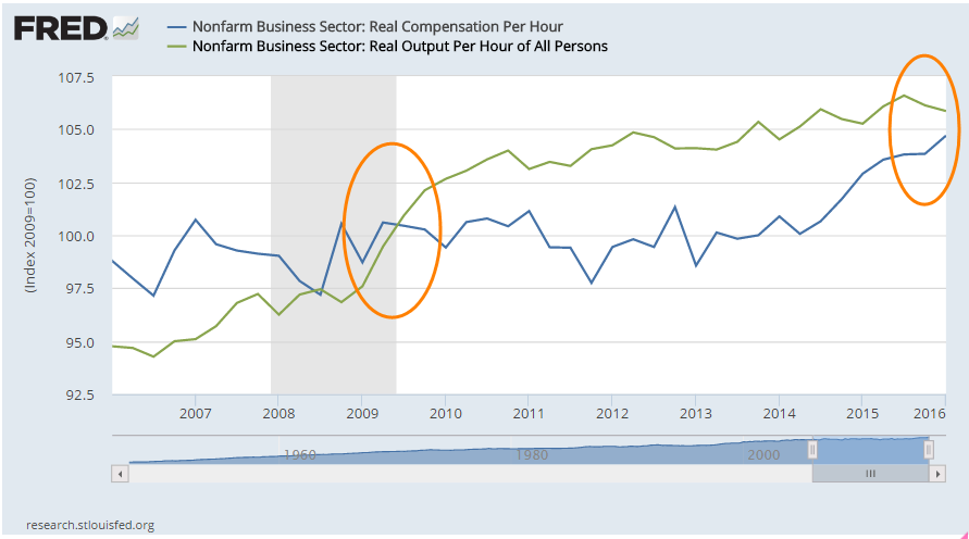
In a recent article, Jim Zarroli with NPR compared productivity growth with the weak growth of only the wages component of employee compensation.  He did leave out an increasingly big chunk of total employee compensation: Federal and State mandated taxes, insurances and benefits.  Since these are mandated costs, the income is not disposable. A term I have never liked for this package of additional costs and benefits is “employer burden.”  The burden is really on the employee as we will see.

In the graph below are two indexes: total compensation per hour and output per hour.  At the end of the last recession in the middle of 2009, the two indexes were the same.  Seven years later, output is slightly higher than total compensation but the discrepancy is rather small compared to the dramatic graph difference shown in the NPR article. As output continues to level and compensation rises more rapidly, we can expect that compensation will again overtake output.

Over the past several decades, employees have voted in the politicians who promised more tax-free insurances and benefits.  While the tax-free aspect of these benefits is an advantage, some employees may think they are freebies.  Payroll stubs produced by more recent software programs enable employers to show the costs of these benefits to employees, who are often surprised at the amount of dollars that are spent on their behalf.  While these benefits are welcome, they don’t pay school tuition, the rising costs of housing or repairs to the family car.

Many voters thought they could have it all because some politicians promised it all: more tax-free insurances and benefits, and higher disposable income.  Total employee compensation, though, must be constrained by productivity growth. In the coming decade, legislators will put forth alternative baskets of total compensation.  More benefits and insurances means less disposable income but a politician can not just say that outright and get re-elected. More disposable income means less insurances and benefits, which will anger other voters.  In short, the political discourse in this country promises to only get more contentious.

Pickup and Letdown

May 8, 2016

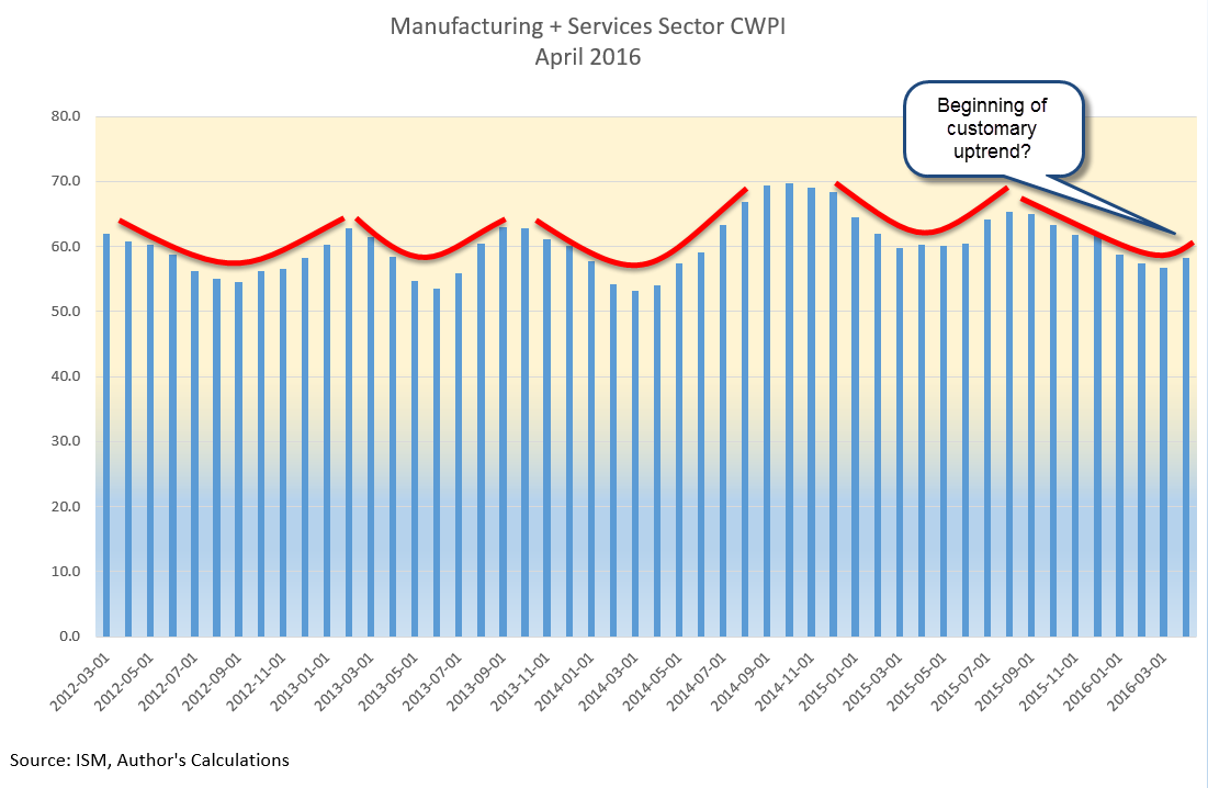
Based on ISM’s monthly survey of Purchasing Managers, the CWPI blends both service and manufacturing indexes and gives additional weight to a few components, new orders and employment.  Last month we were looking for an upward bend in the CWPI, to confirm a periodic U-shaped pattern that has marked this recovery. This month’s reading did swing up from the winter’s trough and we would expect to see further improvement in the coming few months to confirm the pattern. A break in this pattern would indicate some concern about a recession in the following six months. What is a break in the pattern? An extended trough or a continued decline toward the contraction zone below 50.

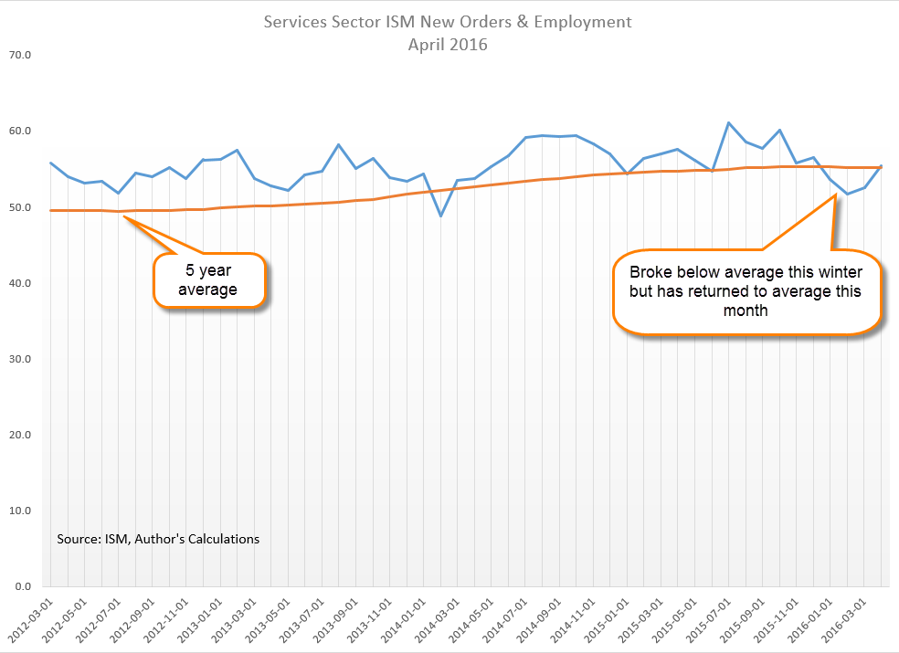
Since the services sectors constitutes most of the economy in the U.S., new orders and employment in services are key indicators of this survey.  A sluggish winter pulled down a composite of the two but a turn around in April has brought this back to the five year average.

Rising oil prices have certainly been a major contributor to the surge in the prices component of the manufacturing sector survey. The BLS monthly labor report (below) indicates some labor cost increases as well.  Each month the ISM publishes selected comments from their respondents.  An employer in the construction industry noted a severe shortage of non-skilled labor, a phenomenon we haven’t seen since 2006, at the height of the housing bubble.

Last week the BEA released a first estimate of almost zero growth in first quarter GDP, confirming expectations.  Oddly enough, the harsh winter of 2015 provided an even lower comparison point so that this year’s year over year growth, while still anemic, is almost 2%.

////////////////////////////

Employment

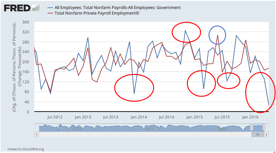
April’s employment data from the BLS was a bit disheartening.  Earlier this week, the private payroll processor ADP reported job growth of 150,000 in April and lowered expectations for the BLS report released on Friday.  While the BLS estimate of private job growth was slightly better, the loss of about 10,000 government jobs, not included in the ADP estimate, left the total estimate of jobs gained at 160,000. The loss of government jobs is slight compared to the total of 22 million employed at all levels of government but this is the fourth time in the past eight months that government employment has declined.

A three month average of job growth is still above 200,000, a benchmark of labor market health that shows job growth that is more than the average 1% population growth  With a base of 145 million employees in the U.S, a similar 1% growth rate in employment would equal 1.5 million jobs gained each year, or about 125,000 per month.  To account for statistical sampling errors, the churn of businesses opening and closing, labor analysts add another 25,000 to get a total of 150,000 minimum monthly job gains just to keep up with population growth.  The 200,000 mark then shows real economic growth.  In March 2016, the growth of the work force minus the growth in population was 1.2%, indicating continued real labor market gains.

Job growth in the core work force aged 25 -54 remains above 1%, another good sign.  It last dipped briefly below 1% in October.  This core group of workers buys homes, cars, and other durable goods at a faster pace than other age groups; when this powerhouse of the economy weakens, the economy suffers. In the chart below, there is an almost seven year period, from June 2007 through January 2014 where growth in this core work force group was less than 1%.  From January 2008 through January 2012, growth was actually negative.  The official length of the recession was 17 months, from December 2007 through June 2009.  For the core work force, the heart of the economic engine, the recession lasted much longer.

In 2005, a BLS economist estimated that the core work force would number over 105 million in 2014.  In December 2014, the actual number was 96 million, a shortage of 9 million workers, or almost 10% of the workforce.  In April 2016, the number was almost 98 million, still far less than expectations.

Some economists and pundits mistakenly compare this recovery from a financial crisis with recoveries  from economic downturns in the late 20th century.  For an accurate comparison, we must look to a previous financial, not economic, crisis – the Great Depression of the 1930s.

The unemployment rate in April remained the same, but more than a half million people dropped out of the labor force, reversing a six month trend of declines.  It is puzzling that more people came back into the labor force during the winter even as GDP growth slowed.

Average hourly earnings increased for the second month in a row, upping the year over year increase above 2.5%.  For the past ten years, inflation-adjusted weekly earnings of production and non-supervisory workers have grown an anemic .75% per year.  In the sluggish winter of January and February 2015, earnings growth notched  a recovery high of 3%, leading some economists and market watchers to opine that lowered oil costs, on the decline since the summer of 2014, would finally spur worker’s pay growth in this long, subdued recovery.  A year later, earnings growth is about 1.2%, a historically kind of OK level, but one which causes much head scratching among economists at the Federal Reserve.  When will worker’s earnings begin to recover?

/////////////////////////

Hungry

A reader sent me a link to a CNBC article  on food insecurity in the U.S. The problem is widespread and not always confined to those who fall below the poverty benchmark. Contrary to some perceptions, food insecurity is especially prevalent in rural areas, where food costs can be 50% higher than urban centers.  How does the government determine who is food insecure? The USDA publishes a guide with a history of the project, the guidelines and questions.  To point out the highlights, I’ll include the page links within the document. The guidelines have not been revised since this 1998 revision.

In surveys conducted by the Census Bureau, respondents are asked a series of questions.  The answers help determine the degree of household food insecurity.  The USDA repeatedly emphasizes that it is household, not individual, insecurity that they are measuring.  The ranking scale ranges from 0, no insecurity, to 10, severe insecurity and hunger. An informative graph of the scale, the categories and characteristics is helpful.

In 1995, a low .8 percent were ranked with severe food insecurity (page 14) . To be considered food insecure, a household must rank above 2.3 (household without children), or above 2 .8 (with children) on the scale.  Above that are varying degrees of insecurity and whether it is accompanied by hunger. (Table)

The USDA admits that measuring a complex issue like this one can provoke accusations that the measure either exaggerates or understates the number of households.  What are they measuring?  Page 6 contains a formal definition, while page 8 includes a list of conditions that the survey questions are trying to assess, and that a condition arose because of financial limitations like “toward the end of the month we don’t have enough money to eat well.”

Page 9 describes the rather ugly pattern of progressively worse food insecurity and hunger.  At first a household will buy cheaper foods that fill the belly.  Then the parents may cut back a little but spare the kids the sensation of hunger.  In its most severe stage, all the family members go hungry in a particular day.

Those of you wanting additional information or resources can click here.

////////////////

Earnings

Almost a month ago the giant aluminum manufacturer Alcoa kicked off the first quarter earnings season.  87% of companies in the SP500 have reported so far and FactSet calculates a 7% decline in earnings.  They note “the first quarter marks the first time the index has seen four consecutive quarters of year-over-year declines in earnings since Q4 2008 through Q3 2009.”  Automobile manufacturers have been particularly strong while the Energy, Materials and  Financial sectors declined.  Although the energy sector gets the headlines, there has also been a dramatic decrease in the mining sector.  The BLS reports almost 200,000 mining jobs lost since September 2014.

The bottom line for long term investors: the economic data supports an allocation that favors equities.  The continued decline in corporate earnings should caution an investor not to go too heavily toward the equity side of the stock/bond mix.

/////////////////

(Edited May 11th in response to a reader’s request to clarify a few points.)

Saving Trends

May 1, 2016

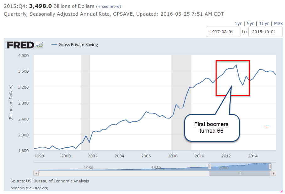
Macroeconomists define saving as Income Less Consumption and Taxes.  There are two distinctions – public, or government savings, and private, or household, savings.

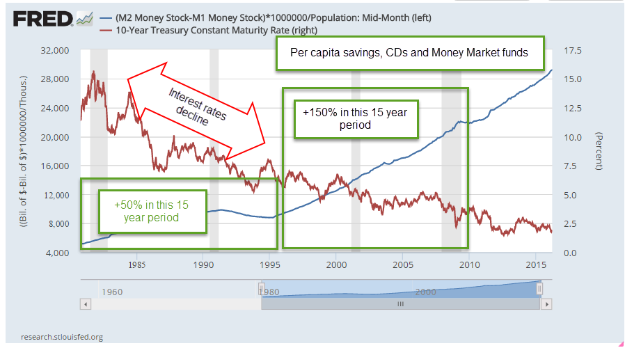
From 1986 to 2000 inclusive, a 15 year period, gross private savings grew 78%.  In the same length of time, from 2001 to 2015, it grew 112%.  So why the higher savings rate?

Lower interest and inflation rates have persisted during this later period.  One would think that consumers would be more likely to save when interest rates were higher in the earlier period.  However, the reverse is true.  Households respond to lower interest rates by saving even more.  Why?  Because their savings will grow more slowly at lower interest rates, they must save more, which only keeps interest rates low.  Like so much of human activity, the process is self-reinforcing.

What else contributes to higher savings rates?  80 million Baby Boomers is more than a third of the population.  As they neared retirement age, they saved more of their income.  In 2012, the first boomers turned 66, a high point in the chart of savings below.

Richard Koo is the chief economist at Nomura, a gigantic Japanese financial holding company similar to Goldman Sachs.  He introduced the idea of a balance sheet recession instigated by a large number of people and businesses paying down their debts to repair their balance sheets.  Here is a recent paper.

Because trends in savings are affected by the decisions of mutiple generations, the primary causes can be difficult to establish.  As the Boomers begin to spend down their savings in retirement, the equally large Millennial generation will start saving but it is unlikely that they will completely offset the spending rate of the Boomers.  The glut of savings will be slowly draw down until new investment puts enough demand for savings, which will spur interest rates higher.

///////////////////

Cadillac Purchasing Power

Last week, I looked at the relative purchasing power to buy a Ford F-150 pickup.  In a trip to a car museum lately, I learned that a new 4 door Cadillac model cost $2000 in 1913.  The average hourly wage was $2 per hour per the NBER, so it took the average person 1000 work hours, about half a year, to buy that Cadillac.  A 2016 Cadillac 4 door ATS Sedan costs about $40,000, an amount that would take 1573 hours, about nine months, at an average $25.43 per hour (BLS).

//////////////////

College Bound

A recent BLS study found that 70% of 2015 HS grads enrolled in college.  Recent NAEP results show that only 37% of test takers are prepared for college reading and math.

//////////////////

Pickup Purchasing Power

April 24, 2016

Relatively stagnant wages and income inequality have become a frequent theme on the campaign trail.  Let’s look at what I’ll call pickup purchasing power to understand the problem.  Sorry.  No graph from the Federal Reserve on this one.

A favorite vehicle among construction workers is the F-150 pickup, a reliable vehicle with room for a toolbox and a trip to the local lumberyard for supplies.  The MSRP of a standard bed 1998 model, available to the public in September 1997, was $14,835 (Source ) In 2016, the MSRP of that same model is $26,430 (Source), a 78% increase, about 3.2% per year.  There have certainly been improvements in that truck model in the past two decades but customers can not order the model without the improvements.  The basic model is the basic model.

Let’s look now at the wages needed to buy that pickup.  In May 1997, shortly before the 1998 F-150 was released to the public, the BLS survey reported average carpenters’ wages of $30,800.  At that time, wages and salaries were about 70.5% of total compensation, or about $43,700 (BLS report).  In the decade before that, wages as a percent of total compensation had declined from 73.3% in 1988 to 70.5% in 1997.  Rising insurance costs and other direct benefits to employees were slowly eating into the net compensation of the average carpenter.

In 2015, the average wage for carpenters was $43,530.  The BLS reported that wages were now 67.7% of the total employment cost, or about $64,300.  In that 18 year period, carpenters’ wages grew 41% but total compensation grew 47%, or 2.1% per year.  The price of that pickup truck, though, grew at 3.2% per year.  That seemingly small difference of 1% per year adds up to a big difference over the years.  That’s the sense of anger that underlies the current election season.  The growth in price of that pickup is only slightly above the average post WW2 inflation rate of 3%.  It is the wages that have fallen behind.

Trump blames the politicians who have given away American jobs with badly negotiated trade agreements that disadvantage Americans.  Trump’s promise to bring those manufacturing jobs back home wins him popular appeal in those communities impacted by the decline in manufacturing.  The loss of manufacturing jobs has left a larger pool of job applicants for construction jobs.  Some of those displaced workers did not have the carpentry skills needed but some were able to work in roles supervised by an experienced carpenter.  The more the supply of job applicants the less upward pressure on wages. If – a big if – some manufacturing jobs do come back to the U.S., it will help spur more growth in carpenter’s wages.

Bernie Sanders blames the fat cats and proposes taxing all but the poorest Americans to distribute income more evenly. His remedies to promote his programs of fairness are far ranging.  Employers who are currently providing health insurance for their employees will probably welcome a 6.2% payroll tax.  On a forty year old employee making $50,000 a year, the $3100 tax is far less cost than an HMO plan. Employers who do not provide such coverage will resent the imposition of more taxes but at least it will be across the board, affecting all competitors within an industry or local market.  Sanders’ healthcare plan also relies on 10% cuts in payments to doctors and hospitals, who are projected to save at least that much in reduced billing costs.

While Trump addresses a specific demographic, a particular segment of the labor market, Sanders proposes broad remedies to a number of problems.  Trump’s appeal will be to those who want a specific fix.  Bring back jobs to our community.  We’ll figure out the rest.  Sanders’ proposals will appeal to voters who have more confidence in government as a problem solver.

///////////////////////////

Oil Stocks

Readers who put some money to work in oil stocks (XLE, VDE for example) in late February, when I noted the historical bargain pricing, might have noticed the almost 20% increase in prices since then.  There are a number of reasons for the surge in price but the buying opportunity has faded with that surge.  Inventories are still high relative to demand.  Recent comprehensive market reports from the IEA require a subscription but last year’s report is available to those interested in a historical snapshot of the supply and demand trends throughout the world.  Until 2014, total demand had slightly exceeded supply.  A glance at the chart shows just how tightly coordinated supply and demand are in this global market. A “glut”in supply may be less than 1% of daily worldwide consumption and it is why prices can shift rather dramatically as traders try to guess both short and long term trends in demand and supply.

Inequality

April 17, 2016

In a 1996 article in Mother Jones magazine economist Paul Krugman (now a N.Y. Times editorial writer) explored the possible causes for growing income inequality.  Yes, twenty years ago income inequality was a “thing.”  A more recent study using hard granular data contradicts a widely held belief that income inequality has grown substantially in the past four decades.

I’ll look first at the older piece by Krugman.  I should note that Krugman was writing for a popular magazine, not an academic journal.  As with his weekly column for the N. Y. Times, Krugman’s goal is to sell his audience a story, to stir up the pot.  Critics who judge an editorial column with the same rigor as an academic paper should be forced to write “I will be kinder to my fellow human beings” one thousand times with a #2 Ticonderoga pencil till they get little pencil indentations in the pads of their fingertips.

Some, including a few contenders in the current Presidential campaign, sound the alarm.  “We’re shipping jobs overseas!”  Well, Krugman considered imports to be a possible cause for inequality but found that imports of goods from third world countries, where wages are markedly lower than the U.S., were only 2% of national income.  Stopping imports from those countries would have but a small effect on workers’ wages.

What about technology? Krugman asked.  As an example of technology, Krugman noted that the educational level of schoolteachers and corporate CEOs are approximately the same yet there is a wide chasm between the compensation of those in these two professions.  If Krugman were my brother-in-law at a Thanksgiving dinner, I’d have argued with him on this one.  “Hey, Paul, whaddayatawkin?!” I would have said, “CEOs are managing way more employees and capital than any teacher!”  Paul would have agreed with me, of course, and apologized for the error of his ways and I would have passed him the cranberry sauce.

 A 2013 study by Faleye, et. al., published in the Journal of Banking and Finance, used a systematic analysis of a salary and pay database to calculate the ratio of CEO pay to the average pay of an employee in the ranks of the company.  They identified and ranked a number of factors to explain the Pay Ratio, as I’ll call it. They found that three factors, ranked in effect, were most important, and by a wide margin:
1) size of the firm, or market cap;
2) tenure of the CEO;
3) return on assets, or profitability of the firm in a given year (Table 3).
Of those three factors, the first two factors, size and longevity, influenced the Pay Ratio far more – three times – than the third factor, the return on assets.

Let’s look at the first factor: the size of the firm.  We’ll use the stock market capitalization (CAP) as an indicator of size.  In the post war period from 1957 to 1980, 23 years, the CAP in the U.S. increased by 2.5 times.  In the subsequent 35 years since 1980, that CAP shot upwards over 13 times, even after two severe market downturns!!

So, CEOs are being paid to be responsible for the deployment of a lot of capital.  Remember, the return on assets (#3 factor) was much less important, so CEOs are being paid even if they don’t do particularly well with that capital in a given year.  Factor #2 was longevity so we can guess that CEOs who do perform well stay in the post.  Those who don’t get the proverbial boot.

Let’s turn to “Fee for service” financial advisors for a comparison.  Advisors typically charge 1 – 2% to manage money for their clients.  Naturally, an advisor – or CEO – who manages a combined $100 million will make more than one who manages $10 million.  The workers at each firm may earn approximately the same but the CEO of the larger firm should make more money and greatly increase the Pay Ratio.

What else can skew the ratio upward?  Using a mean, or average, rather than the median, the halfway number in a data set. The authors of this study found that average CEO pay was almost twice the median CEO pay, indicating that a relatively small number of very well paid CEOs skewed the average upward.  Krugman and other economists (Robert Reich, for example) touting inequality in the popular press use average, not median, CEO pay simply because the average shows a higher ratio than the median. “Whaddayadoin?!” I’d have to challenge Paul at the dinner table.   “In this case, an average gives a distorted view of the data,” I would protest.  Paul might smirk knowingly and grab the last helping of mashed potatoes while I was protesting his dirty, no good argumentative trick.

This study included 447 firms whose total revenues averaged almost $2 billion.  Apple had $600B in revenue last year so the study included both mega firms and large firms.  They found that the median Pay Ratio was 52, not 331 as the AFL-CIO claims, or 150 times, as Krugman claimed in this 1996 article.  Why are there so many different CEO ratios?  The mega companies like Apple, GE and Microsoft will naturally have the highest CEO ratios.  Organizations like the AFL-CIO who want to promote the idea of inequality might use only the pay data from the SP100, the top companies in the world.  In a popular magazine article, the writer doesn’t have to share the characteristics of the data set as one would do in an academic paper so it is relatively easy to convince readers of a particular point of view by careful selection of the data.

As companies have grown in size over the past three decades, the number of named executive officers (NEOs) in each of these large companies have grown.  As companies get bigger, the duties of these NEOs begins to approach that of the CEOs of yesteryear. To compare apples to apples, then, we would do better to compare the salaries of today’s NEOs with the CEOs of 1970. The 2013 study found that the NEO ratio was 23 times the average worker pay, much less than the Pay Ratio of 35 in 1970.  If we average the Pay Ratio (CEO) of 52 in this study and the NEO ratio of 23, we get an average of 37, just about the same as in 1970.

Regardless of the data, most of us are either convinced or not convinced that the Pay Ratio has increased dramatically in the past fifty years.  Our convictions are similar to our tastes – white meat or dark – in turkey.  We can only agree to disagree and know deep down in our hearts that we are, of course, right.

The Weathervane of Growth

April 10, 2016

CWPI (Constant Weighted Purchasing Index)

March’s survey of Purchasing Managers showed a big upsurge in new orders for the manufacturing (MFR) sector. Export orders were up 5.5% in both the manufacturing and services (SVC) sectors and overall output increased 2% or more.  After contracting for several months, MFR employment may have found a bottom.  The total of new orders and employment is still growing but below five year averages.

The broader CWPI is still expanding but at a slightly slower pace for the past seven months.  The cyclic pattern of declining growth followed by a renewal of activity has changed. While there is no cause to make any strategic changes to allocation, it does bear watching in the months ahead.

////////////////////////

IRA Standard of Care

Financial agents – investment advisors, stock brokers and insurance agents – have had different standards of care when they deal with their clients.  The first and highest standard is fiduciary: the agent should operate with the best interests of the client in mind.  Registered Investment Advisors (RIA) are registered with the SEC and follow this strict standard. The second and more lax standard is suitability: the agent should not sell the client anything that is not suitable for the client based on what the client has told them about their circumstances.  Here’s a short paper on the difference between the two standards.

This week the Obama administration issued new guidelines for agents servicing IRA account holders, requiring agents to maintain the higher fiduciary standard starting in 2017.  This requirement was left out of the Dodd-Frank finance reform bill because many in the investment industry lobbied against it.  Here is the first rule proposal in February.

Opponents will criticize the Obama administration for this “new” set of regulations but this policy has been recommended by some in the industry, on both sides of the political aisle, for at least 25 years.  During the 1980s Congress made several changes that made IRA accounts available to a wide swath of savers, most of whom were unfamiliar with the marketplace of financial products now available to them.

Some in the insurance and investment industries fought against the imposition of a stricter fudiciary standard because it would require more training and would likely reduce the sales commissions of agents.  The growing volume of tax deferred employee retirement plans has generated a steady stream of fees for those in the financial industry.

Keep in mind that the new policy only applies to retirement accounts.

////////////////////////

Debt

Banks are in the business of loaning money, meaning that they must loan money to stay in business.  Most of the time some part of the economy wants to borrow money.  Borrowers come in three types:  Household, Corporate and Government.  If households cut back on their borrowing, corporations may increase theirs.

A historical look at total debt as a percent of GDP shows several trends.  Keep in mind the leveling of debt since the financial crisis.  We’ll come back to that later.

In the thirty years following World War 2, debt levels remained fairly consistent with the pace of economic activity.  The three types of borrowers offset each other.  Households and corporations increased their borrowing while government, particularly the Federal government, paid down the high debt incurred to fight WW2.

In 1980 the Reagan administration and a Democratic House began running big deficits, contributing to a spike in the the total level of debt.  By 1993, when President Clinton took office, Federal and State Debt as a percent of GDP was about the same as it was at the end of WW2.

A combination of higher tax rates and cost cutting by a Republican House elected in 1994 led to a reduction in government spending as household and corporations increased their spending.  Total debt levels flattened during the late 1990s.

Following the 9/11 tragedy and a recession, government debt levels increased but now there was no offset in household borrowing as mortgage debt climbed.  Helping to curb the pronounced rise in total debt levels, a Democratic House at odds with a Republican president dampened the growth of government borrowing in the two years before the financial crisis.

Arguably the most severe crisis in eighty years, the financial crisis caused both households and corporations to cut back on their borrowing.  Offsetting this negative borrowing, the Federal government assumed an often overlooked role – the Borrower of Last Resort.  We are accustomed to the role of the Federal Reserve Bank as the Lender of Last Resort, but we might not be aware that some part of the economy has to be the Borrower.  That role can only be filled by the Federal government because the states and local governments are prohibited from running budget deficits.

Look again at the second chart showing the huge spike in government borrowing following the financial crisis.  Now remember the leveling off of total debt shown in the first graph.  The Federal government has increased its debt level by more than $10 trillion.  Almost $4 trillion of that has come from the lender of last resort, the Fed, but the rest of that borrowing has offset a significant deleveraging by corporations and households.  Had the Federal government not borrowed as much as it did, many banks would have experienced significant declines in profits to the point of going out of business.

There is a potential bombshell waiting in the $2 trillion in corporate profits that businesses have parked overseas to delay taxes on the income.  If Congress and the President were to lower tax rates so that corporations could “repratriate” these dollars, two things would happen: 1) corporations could lower their debt levels, using the cash to pay back the rolling short term loans they use to fund daily operations; and 2) the Federal government would lower its debt levels as the corporations paid taxes on those repatriated profits.

Great.  Lower debt is good, right?  Unless households were to step up their borrowing, total debt could fall significantly, causing another banking crisis.  Although politicians on both sides like to talk about bringing profits home, such a move will have to be done slowly so that the economy and the banking system can adjust in slow increments.

Partisans cheer when candidates express strong sentiments in rousing words, but cold caution must quench hot spirits. We can only trust that candidates for public office will temper their campaign rhetoric with prudence if entrusted with the office.

Home Sweet Asset

April 3, 2016

Normally we do not include the value of our home in our portfolio.  A few weeks ago I suggested an alternative: including a home value based on it’s imputed cash flows.  Let’s look again at the implied income and expense flows from owning a home as a way of building a budget.  The Bureau of Labor Statistics and the Census Bureau take that flow approach, called Owner Equivalent Rent (OER), when constructing the CPI, and homeowners are well advised to adopt this perspective.  Why?

1) By regarding the house as an asset generating flows, it may provide some emotional detachment from the house, a sometimes difficult chore when a couple has lived in the home a long time, perhaps raised a family, etc.

2) It focuses a homeowner on the monthly income and rent expense connected with their home ownership.  It asks a homeowner to visualize themselves separately as asset owner and home renter. It is easy for homeowners to think of a mortgage free home as an almost free place to live. It’s not.

3) Provides realistic budgeting for older people on fixed incomes.  Some financial planners recommend spending no more than 25% of income on housing in order to leave room for rising medical expenses.  Some use a 33% figure if most of the income is net and not taxed.  For this article, I’ll compromise and use 30% as a recommended housing share of the budget.

A fully paid for home that would rent for $2000 is an investment that generates an implied $1400 in income per month, using a 70% net multiplier as I did in my previous post. Our net expense of $600 a month includes home insurance, property taxes, maintenance and minor repairs, as well as an allowance for periodic repairs like a new roof, and capital improvements.

Using the 30% rule, some people might think that their housing expense was within prudent budget guidelines as long as their income was more than $2000 a month.  $600 / $2000 is 30%.

However, let’s separate the roles involved in home ownership.  The renter pays $2000 a month, implying that this renter needs $6700 a month in income to stay within the recommended 30% share of the budget for housing expense.  The owner receives $1400 in net income a month, leaving a balance of $5300 in income needed to stay within the 30% budget recommendation. $6700 – $1400 = $5300.  Some readers may be scratching their heads.  Using the first method – actual expenses – a homeowner would need only $2000 per month income to stay within recommended guidelines.  Using the second method of separating the owner and renter roles, a homeowner would need $5300 a month income. A huge difference!

Let’s say that a couple is getting $5000 a month from Social Security, pension and other investment income.  Using the second method, this couple is $300 below the prudent budget recommendation of 30% for housing expense.  That couple may make no changes but now they understand that they have chosen to spend a bit more on their housing needs each month.  If – or when – rising medical expenses prompt them to revisit their budget choices, they can do so in the full understanding that their housing expenses have been over the recommended budget share.

This second method may prompt us to look anew at our choices.  Depending on our needs and changing circumstances, do we want to spend $2000 a month for a house to live in?  Perhaps we no longer need as much space.  Perhaps we could get a suitable apartment or townhome for $1400?  Should we move?  Perhaps yes, perhaps no.  Separating the dual roles of owner and renter involved in owning a home, we can make ourselves more aware of the implied cost of our decision to stay in the house.  A house may be a treasure house of memories but it is also an asset.  Assets must generate cash flows which cover living expenses that grow with the passage of time.

/////////////////////

The Thrivers and Strugglers

“Bravo to MacKenzie. When she was born, she chose married, white, well-educated parents who live in an affluent, mostly white neighborhood with great public schools.”

In a recent report published by the Federal Reserve Bank at St. Louis, the authors found that four demographic characteristics were the chief factors for financial wealth and security:  1) age; 2) birth year; 3) education; 4) race/ethnicity.

While it is no surpise that our wealth grows as we age, readers might be puzzled to learn that the year of our birth has an important influence on our accumulation of wealth.  Those who came of age during the depression had a harder time building wealth than those who reached adulthood in the 1980s.

Ingenuity, dedication, persistence and effort are determinants of wealth but we should not forget that the leading causes of wealth accumulation in a large population are mostly accidental.  It is a humbling realization that should make all of us hate statistics!  We want to believe that success is all due to our hard work, genius and determination.

//////////////////////

Employment

March’s job gains of 215K met expectations, while the unemployment rate ticked up a notch, an encouraging sign.  Those on the margins are feeling more confident about finding a job and have started actively searching for work.  The number of discouraged workers has declined 20% in the past 12 months.

Employers continue to add construction jobs, but as a percent of the workforce there is more healing still to be done.

The y-o-y growth in the core workforce, aged 25-54, continues to edge up toward 1.5%, a healthly level it last cleared in  the spring of last year.

The Labor Market Conditions Index (LMCI) maintained by the Federal Reserve is a composite of about 20 employment indicators that the Fed uses to gauge the overall strength and direction of the labor market.  The March reading won’t be available for a couple of weeks, but the February reading was -2.4%.

Inflation is below the Fed’s 2% target, wage gains have been minimal, and although employment gains remain relatively strong, there is little evidence to compel Chairwoman Yellen and the rate setting committee (FOMC) to maintain a hard line on raising interest rates in the coming months.  I’m sure Ms. Yellen would like to get Fed Funds rate to at least a .5% (.62% actual) level so that the Fed has some ability to lower them again if the economy shows signs of weakening.  Earlier this year the goal was to have at least a 1% rate by the end of 2016 but the data has lessened the urgency in reaching that goal.

ISM will release the rest of their Purchasing Manager’s Index next week and I will update the CWPI in my next blog.  I will be looking for an uptick in new orders and employment.  Manufacturing lost almost 30,000 jobs this past month – most of that loss in durable goods.  Let’s see if the services sector can offset that weakness.

///////////////////////////

Company Earnings

Quarterly earnings season is soon upon us and Fact Set reports that earnings for the first quarter are estimated to be down almost 10% from this quarter a year ago.  The ten year chart of forward earnings estimates and the price of the SP500 indicates that prices overestimated earnings growth and has traded in a range for the past year.  March’s closing price was still below the close of February 2015.  Falling oil prices have taken a shark bite out of earnings for the big oil giants like Exxon and Chevron and this has dragged down earnings growth for the entire SP500 index.

Dynamic Portfolio Allocation

March 27, 2016

Happy Easter!

Before I take a look at a dynamic allocation model for older readers, I’ll quote from a paper published in the last decade: “adequate savings is the primary driver of retirement success and is approximately 5 times more important than Asset Allocation.”  For readers who are not near retirement, what is called the accumulation phase of life, the one word that sums up a lot of financial advice is “Save.”

A reader sent me an article that recounts several common sense strategies for investors nearing or in retirement.  I was especially interested in a strategy for recent retirees: to have a cautious 30/70 stock/bond allocation in the first years of retirement and transition to a more agressive 60/40 portfolio over 10 – 15 years. Is this madness?  Conventional advice advocates more caution in the later years of life.

The initial conservative approach is designed to minimize the negative effects that a bear market would have on a portfolio in the first years of retirement.  At seven years old, the current bull market is long in the tooth, so to speak. One of the authors of the article is Wade Pfau, whose Retirement Researcher site I include in my blog links in the right column of this blog.  I have a lot of respect for Mr. Pfau’s work and his sensibilities so I was inclined to trust this recommendation.

In order to forecast, one has to backtest, and the authors have more sophisticated portfolio allocation testers than many of us have.  I have recommended before a free allocation tester at Portfolio Visualizer.  Their web site also has a free Monte Carlo simulation tool (MC).  What the heck is that, you ask?

For Dr. Who fans, an MC is like a time trip in the doctor’s Tartus.  First we set the thing jab on the whozee panel, spin the furbee wheel clockwise to go forward in time, then stand one pace to the left – do not stand on the right! – of the big lever as we pull the lever knob.

For those of you without a Tartus, an MC uses historical returns and creates a number of what-if possibilities based on variable parameters like the period of time to run the simulation, the inflation rate, the withdrawal amount or rate, the asset mix, etc.  If I start out with $1M in savings at age 65, for example, and I take out $40,000 each year adjusted for inflation, what are the chances I will have any money left after thirty years, at age 95?  Will the Daleks catch up with my savings and exterminate it?  No, not the Daleks!

The remaining balance, the money a person would have left, is ordered by percentile: 25%, 50%, the median, and 75% are common. Example:  A remaining balance of $500K for a certain allocation at the 75% percentile means that 75% of retirees will have less than that amount.

A success rate is computed; a 75% success rate means that you don’t run out of money in 75% of the simulations.  What about the other 25% of the time?  Care to roll the dice on that one? A 90% success rate is considered a desireable minimum in the industry.  I tend to focus on both the success rate and the median balance.

If using historical asset prices as a basis for computing future possibilities, an important assumption is the time period.  If the past forty years have included some really good returns for a few decades, then the MC results will be optimistic.  What if the next twenty years are not so good?  Move in with your kids?

Using the historical data of the past 20 years or 40 years as a basis for future returns is a bit optimistic, I think.  During this past twenty years, bond prices have been inflated by extraordinarily low interest rates set by the Federal Reserve.  The price of a composite of intermediate corporate bonds, Vanguard’s VFICX mutual fund, has almost quadrupled since 1995.  A 60/40 stock/bond mix has returned 9.5% over the past 20 years.  We are unlikely to see such returns in the future.  My gut instinct is to err on the side of caution and assume a 7.5% return on a 60/40 mix, and a 6% return on a 30/70 mix.

Here’s the assumptions:  $1M initial portfolio; 30 year future period; withdraw an initial $45K adjusted annually using a 3% inflation rate.

.nobrtable br { display: none } td {text-align: center;}

Stock/Bond % Success Rate Median Bal
30/70 57 $278K
60/40 73 $1.6M
30/70 –> 60/40 92 $1.7M

Using a 30/70 mix for the first 5 years and a 60/40 mix for the following 25 years gives a median balance of $1.7M after 30 years, about the same as the 60/40 mix above BUT the success rate shoots up to 92%.   The authors suggest a gradual transition but this simple simulation shows the advantage of a dynamic allocation strategy.

In short, this does look like a good strategy.

Readers who want to use the more optimistic historical returns of the past 20 years would see these simulation results:

Stock/Bond % Success Rate Median Bal
30/70 92 $2.7M 10 times higher!
60/40 88 $4.3M
30/70 –> 60/40 92 $4.3M

Using historical returns for the past 20 years sure pumps up the median balance on the conservative allocation.

///////////////////

Existing Homes

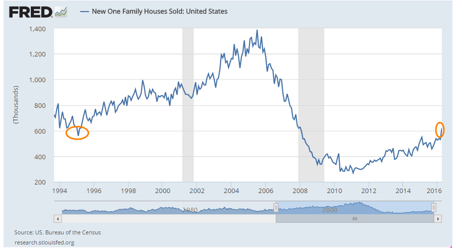
Existing Home sales fell 7% in February.  Mortgage rates are at all time lows.  What’s going on?
Below is a chart of the ratio of Existing Home Sales to New Single Family Homes.  As you can see, the ratio has remained fairly steady over the past several years.  The spike in the ratio in early to mid 2013 coincided with historically low mortgage rates (Money) .   In the last quarter of 2015, this ratio started sinking despite the stimulus of low interest rates.  Are home buyers at all levels being priced out of the market?

////////////////////////

The Immigration Carousel

The 1900 census counted a total population of 78 million, of which 13% were foreign born. Responding to a growing hostility toward immigrants, Congress passed strict quota laws for immigrants in 1921 and 1924. Regarded as lazy, shiftless, boorish, stupid, or criminal, southern Europeans were among the undesireable groups.  During the 1920s, the foreign born population began to decline and, beginning with the 1950 census, stayed below 8% for 40 years.

The 2000 census counted 11% of the population as foreign born. The 2010 census counted 13% foreign born, so that our population mix now matches that of the early 20th century.

It is hardly surprising then to see a growing antipathy towards immigrants in the past decade.  Donald Trump’s candidacy is partly fed by the same anti-immigrant sentiment prevalent in the America of one hundred years ago.  We like to think we have put some crude and cruel instincts behind us, but we are again confronted with our “herdness.”  We will tolerate “others” as long as their percentage of the herd remains relatively small. In America, that tolerance limit seems to be 10% foreign born. How does America compare to other countries?

The Donald and the Washington Post

March 22, 2016

The editorial board and several other employees at the Washington Post recently sat down with Donald Trump.  Here is a transcript of the conversation .

Here are some highlights.   Donald rambles a lot but I think I got the kernel of his responses.  I think my edited version does Donald more justice than the sometimes incoherent responses he actually gave. He really is not ready for prime time. At this point in the campaign his responses to questions about foreign policy, international trade, and other issues mentioned on the campaign trail should be more practiced, not the rambling sentiments that any of us might have in a conversation with a co-worker at a lunch break.

WP = Editorial staff at Washington Post, DT = Donald Trump.  I’ve included some context where I thought it might be needed.

WP: “is there a secretary of state and a secretary of defense in the modern era who you think have done a good job?”

DT: “I think George Shultz [Reagan’s Sec’y State] was very good, I thought he was excellent.”  “I think your last secretary of state [Hillary Clinton] and your current secretary of state [John Kerry] have not done much.”  Trump uses the word “your” to indicate that media institutions are partisan and biased, and including the WP in the liberal media. It indicates that Trump’s essential sense of the world is polarized, a game of warball.  That may be the case in Washington but it mutes Trump’s appeal among independent voters who have less polarized outlooks. Trump offered an example of Kerry’s bad negotiating tactics with Iran: “We should have had our prisoners before the negotiations started.”

In response to a question about promoting values like democracy and freedom around the world,
DT: “I don’t think we should be nation building anymore,” indicating that he is not a neo-con. “We’re sitting probably on a bubble and, you know, it’s a bubble that if it breaks is going to be very nasty. And I just think we have to rebuild our country.”   Trump is not the only person who thinks that extremely low interest rates for seven years have over inflated stock, bond and housing values.  Trump immediately changes the subject and endorses infrastructure spending, aligning himself with economists Paul Krugman, Robert Frank, and others who recommend large Federal stimulus programs to repair infrastructure and employ those with low to modest educational backgrounds.  Trump recalls that we built schools in Iraq, and rebuilt them several times when they got bombed “and yet we can’t build a school in Brooklyn. We have no money for education, because we can’t build in our own country. And at what point do you say hey, we have to take care of ourselves. “

WP: “So what would you do for Baltimore [as an example of a city with troubled inner neighborhoods]”

DT: “I’d create economic zones. I’d create incentives for companies to move in. I’d work on spirit because the spirit is so low… unemployment for black youth in this country, African American youth, is 58-59 percent.”  These are called enterprise zones and have been used with mixed success in the U.S. but particularly in Britain.  See this article

WP: “in general, do you believe there are disparities in law enforcement?”

DT: “I’ve read where there are and I’ve read where there aren’t…I have no opinion on that.  We have to create incentives for people to go back and to reinvigorate the areas and to put people to work…we have lost million and millions of jobs to China and other countries.”   When Trump doesn’t like the topic, law enforcement, he switches subjects to an old refrain, jobs lost to China, and now Mexico. “Mexico is really becoming the new China.”

WP, returning to the topic:  “There is disproportionate incarceration of African Americans vs. whites. Is that something that concerns you?”

DT: “It would concern me. But at the same time it can be solved to a large extent with jobs.”  Some economists and social scientists have championed this idea that people in poor neighborhoods will choose  legal employment if presented with better job prospects.  Over time, residents in the area will become more committed to the neighborhood, to the protection of their property, to law and order.

WP: “Baltimore received a lot of federal aid over the years. What’s different specifically about your approach to these issues from what’s been tried in the past, because a lot of effort has been put in just the direction you just described.”

DT: “I think what’s different is we have a very divided country.”  He goes on about how divided the country is, as if we didn’t already know that.  How does that answer the question about Baltimore? “I thought that President Obama would be a great cheerleader for the country. And it just hasn’t happened. You have to start by giving them hope and giving them spirit and that has not taken place. I actually think I’d be a great cheerleader for the country.”

WP: “What presidential powers and executive actions would you take to open up the libel laws?”

DT: “I’ve had stories written about me … that are so false, that are written with such hatred.  I think libel laws almost don’t exist in this country.  I think that [the media] can do a retraction if they’re wrong. They should at least try to get it right. And if they don’t do a retraction, they should, they should you know have a form of a trial. I don’t want to impede free press, by the way.”

WP: “So in a better world would you be able to sue [the Post]?”

DT: “In a better world I would be able to get a retraction or a correction. Not even a retraction, a correction.”

WP: “Would you require less than [actual] malice for news organizations?”  “Actual malice” is a legal standard, a criteria for liability for libel set up the Supreme Court in 1964.  See below.

DT: “I would make it so that when someone writes incorrectly, yeah, I think I would get a little bit away from malice without having to get too totally away.”  What does that mean?

WP: “How are you defining ‘incorrect?’ It seems like you’re defining it as fairness or your view of fairness rather than accuracy.”

DT: “Fairness is… part of the word. I’ve had stories that are written that are absolutely incorrect. I’ll tell you now and the word ‘intent’, as you know, is an important word, as you know, in libel.”  Trump then gives an example of a news account of a protester at a Trump rally.  The video tape is edited to make Trump supporters look guilty of unprovoked violence.  Trump says these are professional protesters with trained voices that can be heard throughout a large hall in order to disrupt Trump’s speech or a question from the crowd.  Trump says that news media accounts do not potray these incidents accurately.

Through several questions various people from the Post try to get Trump to acknowledge that Trump condones violence.  Trump insists that he supports law and order, not violence.  Trump’s campaign manager notes that there are repeated public service messages before every rally that the audience should not confront protestors and to let security personnel do that.  Trump repeats that some protesters, when interviewed, say they don’t know why they are there, implying that the protesters are paid agitators by those who want to make Trump rallies look violent.  Some protesters simply interrupt his speeches with shouted obscenities.  Out of 20,000 attending a rally, Trump claims that there are just a few protesters and that they are strategically placed at the rally venue.

WP:  “given the Supreme Court rulings on libel — Sullivan v. New York Times — how would you change the law?”  New York Times v. Sullivan is a 1964 decision by the Supreme Court that there must be a malice standard applied before reporting about a public official can be considered libel.  “Actual malice” is a legal concept that the media outlet knew the information was incorrect or should have known, i.e. that they exercised little or no effort to find the correct information.  After this decision, a person claiming libel in the U.S. must prove the untruth of something published.  This departed from centuries of common law precedent.  In Britain, for example, the defendant of a libel claim must prove the truth of the information they published.

DT: “I’d have to get my lawyers in to tell you, but I would loosen them up.”  Although Trump is not specific on this, I’m guessing that he would like some balance between the strict U.S. system and the Briitish system.  U.S. precedent was based on a problem that existed in the southern states during the early 20th century.

WP: “Would that be the standard then? If there is an article that you feel has hatred, or is bad, would that be the basis for libel?”

DT: “The Washington Post never calls me. I never had a call, ‘Why – why did you do this?’ or ‘Why did you do that?’ It’s just, you know, like I’m this horrible human being. And I’m not.”  If a news organization makes no effort to validate information, is that cause for libel?  “I want to make it more fair from the side where I am, because things are said that are libelous, things are said about me that are so egregious and so wrong, and right now according to the libel laws I can do almost nothing about it because I’m a well-known person.”

WP: “can you talk a little bit about what you see as the future of NATO? Should it expand in any way?”

DT: “Ukraine is a country that affects us far less than it affects other countries in NATO, and yet we are doing all of the lifting, [European members of NATO are] not doing anything.”

WP: “Could I ask you about ISIS, speaking of making commitments, because you talked recently about possibly sending 20 or 30,000 troops”

DT: “I said the generals, the military is saying you would need 20- to 30,000 troops, but I didn’t say that I would send them. I would put tremendous pressure on other countries that are over there to use their troops and I’d give them tremendous air … support because we have to get rid of ISIS. I would get other countries to become very much involved.”

WP: “What about China and the South China Sea?”

DT: “We have trade power over China. I don’t think we are going to start World War III over what they did, it affects other countries certainly a lot more than it affects us. I always say we have to be unpredictable. We’re totally predictable.  And predictable is bad. Sitting at a meeting like this and explaining my views and if I do become president, I have these views that are down for the other side to look at, you know. I hate being so open.”

WP:  Asks about Iraq and ISIS

DT: “We then got out [of Iraq] badly, then after we got out, I said, “Keep the oil. If we don’t keep it Iran’s going to get it.” And it turns out Iran and ISIS basically—”  Trump is interrupted but I wonder if he was going to say that Iran and ISIS were conspiring to get Iraq’s oil?  Iran and ISIS are blood enemies.  Iran embodies the Shia sect of Islam, ISIS is Sunni.

WP: “How do you keep it without troops, how do you defend the oil?”

DT: “I would defend the areas with the oil [with U.S. troops].”  Asserting that Iran is out for Iraq’s oil, Trump says, “Iran is taking over Iraq as sure as you’re sitting there. And I’ve been very good on this stuff. My prognostications, my predictions have become, have been very accurate, if you look.”

WP:  Asks Trump about his claim that he could use trade as a diplomatic cudgel against China’s territorial ambitions in the South China sea.  These disputes involve Vietnam, the Phillipines, and Malaysia.

DT: “You start making it tougher [for Chinese exporters]. They’re selling their products to us for… you know, with no tax, no nothing. If you’re a manufacturer, you want to go into China? It’s very hard to get your product in, and if you get it in you have to pay a very big tax.” “I don’t like to tell you what I’d do, because I don’t want to…”

WP: “This theory of unpredictability …there are many people who think that North Korea invaded South Korea precisely because [Secretary of State Dean] Acheson wasn’t clear that we would defend South Korea. So I’m curious, does ambiguity sometimes have dangers?”  Acheson served under Truman from 1949 to 1953.  In 1950, the N. Korean People’s Army crossed the 38th parallel to invade South Korea.

DT: “President Obama, when he left Iraq, gave a specific date – we’re going to be out. I thought that was a terrible thing to do. [The enemy] pulled back, and after we left, all hell broke out, right?”

WP: “What you’re saying [about European NATO members] is very similar to what President Obama said to Jeffrey Goldberg (Atlantic article) in that we have allies that become free riders. Do you have a percent of GDP that they should be spending on defense? Because it’s not that you want to pull the U.S. out [of NATO].”

DT:  “No, I don’t want to pull it out. NATO is costing us a fortune and yes, we’re protecting Europe but we’re spending a lot of money.”  Again, nothing specific in answer to the question.

WP:  “does the United States gain anything by having bases [in Japan and S. Korea]?”  The Post cites an unnamed public source that the U.S. pays 50% of non-personnel costs to maintain the bases.

DT: “I think we were a very powerful, very wealthy country. And we’re a poor country now. We’re a debtor nation.  We’re spending that [money] to protect other countries. We’re not spending it on ourselves. We have armor-plated vehicles that are obsolete. The best ones are given to the enemy.”  Donald relates that the son of one of his friends has served three tours in Iraq and Afghanistan.  “He said the enemy has our equipment – the new version — and we have all the old version, and the enemy has our equipment.  “We send 2,300 Humvees over, all armor-plated. we have wounded warriors, with no legs, with no arms, because they were driving in stuff without the armor. And the enemy has most of the new ones we sent over that they captured. And he said, it’s so discouraging when they see that the enemy has better equipment than we have – and it’s our equipment.”

There was more, including someone at the Post asking about the size of Donald’s hands.

Free Trade

March 20, 2016

This week’s blog will be about free trade.  Donald Trump first made it one of two signature Presidential campaign issues, then Bernie Sanders joined the chorus and now Hillary Clinton has made it part of her campaign speech. Have trade agreements with other countries put Americans at a disadvantage?

Most economists will not even entertain the idea.  The benefits of free trade are ultimately based on the benefits of specialization, the idea that everyone benefits when the most efficient producers supply a good or service.  Each producer achieves a comparative advantage (CA) in that specialization.   First formalized by economist David Ricardo in the 19th century, CA has long been a bedrock of micro-economic theory and introductory economics textbooks.

Greg Mankiw’s Prinicples of Economics cites the example of a rancher and farmer, who both benefit when they specialize.  The rancher concentrates on raising beef, the farmer raises potatoes and they produce more beef and potatoes at a lower cost than if the rancher and farmer did both. (Chapter 3)

A key concept to understanding CA is another bedrock economic principle:  opportunity cost, or what someone has to give up (the cost) to get some good or service (opportunity).  Each person, each country wants to minimize the cost to take advantage of the opportunity.

The same principle can be extended to international trade.  If a Mexican company can produce a good at a more efficient cost than an American company, then Americans will benefit if they buy the good from Mexico and sell something to Mexico which an American company can produce at a cheaper cost.  The ill effects in a particular part of the country are balanced by the good effects in another part of the country or economy, and lower prices benefit all Americans.

When countries impose tariffs on imports, those goods become more expensive for consumers. Economists talk about the “deadweight loss” from tariffs. Here is a graph of the negative effects of tariffs and more discussion on the topic.

The matter would seem settled then, as economist Paul Krugman noted in a 1987 paper : “the underlying commonality among conventional trade models is such that until a few years ago international trade theory was one of the most unified fields in economics.”

As early as the 1960s, economists questioned some aspects of conventional trade models, leading to the development of new models. Krugman notes, “The new view of international trade holds that trade is to an important degree driven by economies of scale rather than comparative advantage, and that international markets are typically imperfectly competitive.” [my emphasis]

Economies of scale. What’s that? This idea, also called increasing return, is when a producer gets a greater growth in outputs than the growth in inputs.  Increasing returns become a force separate from comparative advantage that leads to a “geographical concentration of production of each good,” or regional oligopolies.  We see this phenomenon in southeast Asia, Indonesia and Australia, where a complex web of materials and components production dominates the global electronics market.

“The view that free trade is the best of all possible policies is part of the general case for laissez-faire in a market economy, and rests on the proposition that markets are efficient. If increasing returns and imperfect competition are necessary parts of the explanation of international trade, however, we are living in a second-best world where government intervention can in principle improve on market outcomes.” [my emphasis]  The new idea in trade models is that strategic trade policy by a government “can tilt the terms of oligopolistic competition to shift excess returns from foreign to domestic firms.”  On the campaign stump, Trump makes the same case, although a bit less elegantly; that the U.S. government should make trade deals that shift the benefits of trade back to American workers and producers.  Is Trump channeling Paul Krugman?

Not quite.  Krugman notes three sometimes vociferous criticisms of government intervention. 1) The difficulty in measuring, understanding and modeling imperfect markets makes it impossible to formulate just the right policy.  2) If the government is going to intervene, companies will devote some resources to compete for favors from government, a process called “rent-seeking.” 3) Markets will make adjustments to offset intervention.  Other governments will initiate policies to counter the effects of a government’s intervention.

Krugman concludes “This is not the old argument that free trade is optimal because markets are efficient. Instead, it is a sadder but wiser argument for free trade as a rule of thumb in a world whose politics are as imperfect as its markets.”  This is the argument that Adam Smith made for laissez-faire capitalism, finding it undesireable but better than the alternatives.  Smith spent considerable effort in his book The Wealth of Nations to recount the degree of political corruption that distorted economies and society, that poisoned the human character.

That Krugman disregards those cautions when he favors government intervention within domestic markets confirms the fact that economists are human.

Economist Ian Fletcher presents far more arguments against free trade than Krugman. I would add an additional consideration.  When economists compute the costs of free trade policies, they use a model which does not include the economic benefits provided to workers displaced by free trade policies.  The costs are presumed to be offset by higher taxes from those areas of the country which benefit from free trade.  Admittably, these costs and additional tax revenues attributable to free trade policies are difficult to measure.  However, I do think that the effort should be made.  I suspect that the benefits paid to dislocated workers and the total negative effect, the multiplier, of the lost economic activity have not been fully accounted for and that free trade is much more costly than conventional models portray.

Even if we can measure and agree on the facts, we can not agree on what those facts mean.  Whatever the facts, we prefer our familiar and favorite idea.  They not only reassure us but are also well integrated into our values, and our philosophical sense of life.