February 28, 2016
Heaven on Earth
The tax and spending policies proposed by Presidential contender Bernie Sanders were “vetted” by economist Gerald Friedman. David and Christina Romer review Friedman’s assumptions and methodology, finding the former unrealistic and the latter flawed. Christina Romer was former chair of the Council of Ecomic Advisors during the Obama administration.
Friedman assumes that Sanders’ income redistribution policies will spur a lot of demand in the next decade, 37% more than the Congressional Budget forecasts. Real GDP will grow by 5.3% per year (page 7), erasing the effects of the 2008 financial crisis. Friedman also thinks that the productive capacity of this country is far below its optimum. Therefore, all that extra demand will not lead to increased inflation, which would naturally put a brake on economic growth. Employment will increase by 26% from the 2007 peak and, magically, all that extra demand for workers will not cause an increase in wages and inflation.
On page 8, the authors provide some historical context: “Growth above 5% has certainly happened for a few years, such as coming out of the severe 1982 recession. But what Friedman is predicting is 5.3% growth for 10 years straight. The only time in our history when growth averaged over 5% for a decade was during the recovery from the Great Depression and the years of World War II.”
While GDP growth averaged over 5% during the decade after WW2, it was erratic growth spurred on by the inability of many families to buy many household items during the war. It included one recession as well as phenomenal growth of 13% in 1950, and is unlikely to be replicated.
But we want to believe, don’t we?
/////////////////////
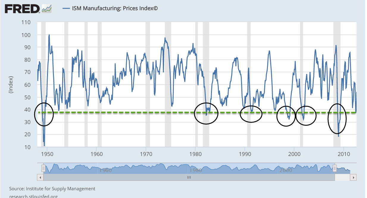
Labor Force Health Report
Yes, we’re busy so who has time to look at a lot of data to understand whether the world will implode tomorrow? As an indicator, the health of the labor market is pretty good. To take the temperature of the labor market we can look at the ratio of active job seekers to job openings. At an ideal level of 100%, seekers = openings. In the real world, there are always more job seekers than job openings. When the percentage of seekers to openings is 200%, it is almost certainly a recession. The economy rarely produces levels below 150%, which means that there are 3 job seekers for every 2 job openings.

Looks pretty good on a historical basis, doesn’t it?
///////////////////
Women in the Workforce
Fact Check: Women make less than men. In 2013, the BLS published a survey comparing the full time wages of men and women in the general population and by race. In 2012, median weekly earnings for women were 81% of men’s. Black and Hispanic women were higher, at 90% and 88%, but this may be due to the fact that Black and Hispanic men make less than white men.
Education levels have changed dramatically. In 1970, only 11% of women had a college degree. In 2012, 38% did, just slightly below the 40% average for the U.S. A 2010 BLS study found that, in 2009, median weekly earnings of workers with bachelor’s degrees were 1.8 times the average amount earned by those with a high school diploma. (They are comparing a median to an average to reduce the effect of especially high incomes).
What the BLS notes is that “the comparisons of earnings in this report are on a broad level and do not control for many factors that may be important in explaining earnings differences.” We will never hear that on the campaign trail. Academic caveats do not get voters fired up to go out and vote. If a candidate is running on a platform of fixing income disparity (Democrats), we will hear quoted the report with the most disparity. Candidates running who claim little disparity (Republicans) will quote a paper whose statistical assumptions minimize income differences.
A more distressing trend is that older women are having to work longer. 8% of women worked beyond retirement age in 1992. The percentage has almost doubled to 14%. The BLS estimates that, in ten years, 20% of women will be working past retirement age.
///////////////////////////
Oil Rig Count
Almost half of the oil and gas rigs in the U.S. are located in Texas. The 60% reduction in Texas rigs reflects the decline in total rigs throughout the U.S., according to Baker Hughes. Rigs pumping oil account for 3/4 of the rigs shut down.

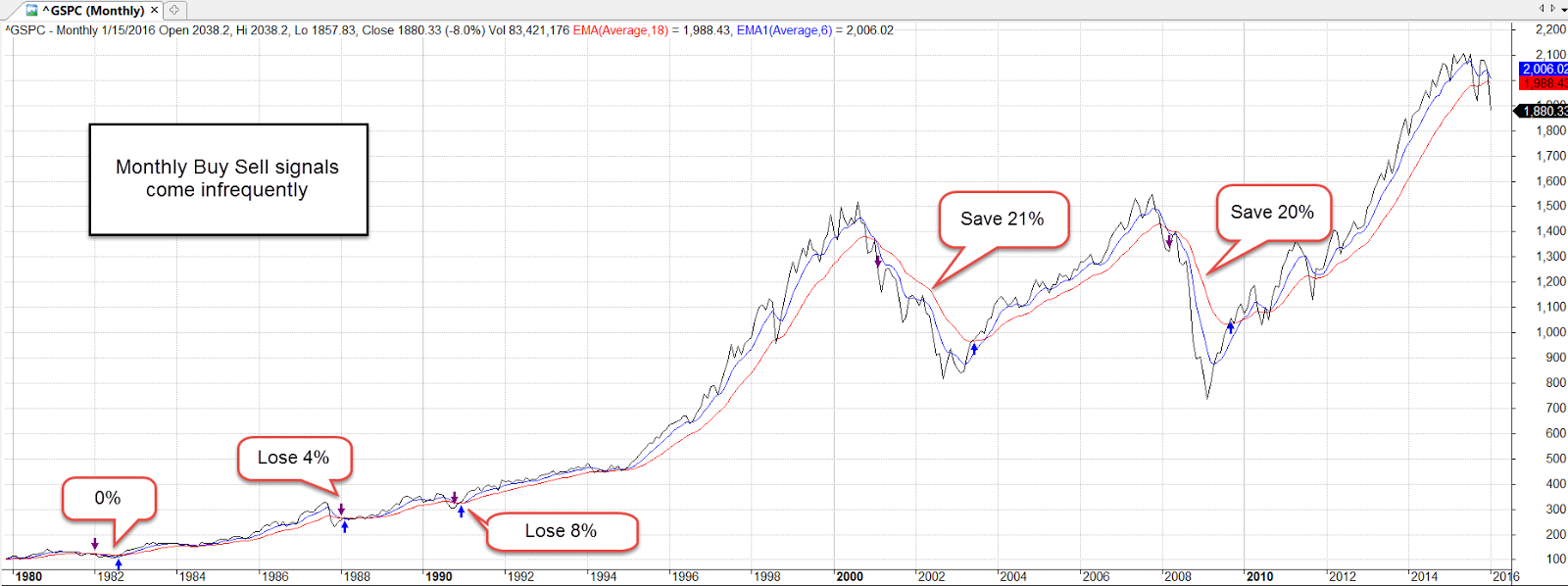
The oil “glut” is only about 1.5 million barrels of oil per day, less than 2% of the 2016 daily demand of 96 million gallons barrels estimated by the IEA. Fewer rigs reduce downward price pressures and lately we have seen crude prices rise into the mid-$30s. With a long time horizon of several years or more, a diversified mutual fund or ETF like XLE, VDE or VGENX would likely provide an investor with some dividend income and capital gains. Could prices go lower? Of course. After falling more than 40% in 2008, the SP500 stood at 900 at the end of December. Investors who bought at those depressed levels might have felt foolish when the index dropped another 25% in the following months. Those “fools” have more than doubled their investment in the past 7 years, averaging annual gains greater than 12%.